5 Ways to Apply Conditional Formatting Between Excel Sheets

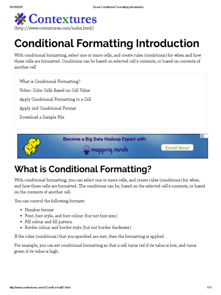
Conditional formatting is a powerful feature in Excel that helps users visualize data and identify patterns by automatically applying formatting based on cell values. While many users are familiar with applying conditional formatting within a single sheet, it's often not as widely known how to effectively utilize this tool across multiple sheets. Here, we'll explore five effective ways to apply conditional formatting between Excel sheets, ensuring your data is consistently formatted and easily interpretable across your entire workbook.
Method 1: Using the INDIRECT Function

The INDIRECT function can be quite useful when you need to reference a range in another sheet dynamically. Here’s how to use it for conditional formatting:
- Select the range in your current sheet where you want the conditional formatting to apply.
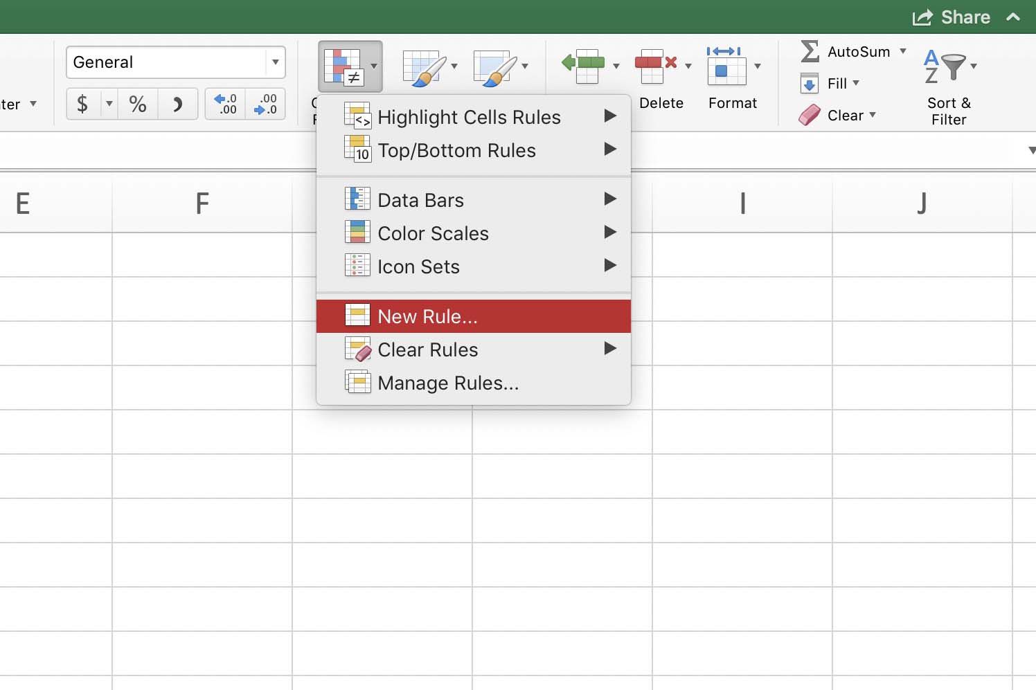
- Go to the ‘Home’ tab, click on ‘Conditional Formatting’, then choose ‘New Rule’.
- Select ‘Use a formula to determine which cells to format’.
- Enter the following formula:
=INDIRECT(“Sheet2!A1:A10”)=INDIRECT(“Sheet1!” & ADDRESS(ROW(),COLUMN()))This formula assumes you’re checking if cell values in Sheet1 match those in a corresponding range in Sheet2. - Click ‘Format’ to choose how you want cells to be highlighted if the condition is met, and then hit ‘OK’.
This method allows for dynamic referencing which is particularly useful when sheet names or the location of data might change.
⚠️ Note: Ensure the sheet names referenced in the formula exactly match the names of your actual sheets.
Method 2: Creating Name Ranges for Referencing

Using named ranges can make your conditional formatting formulas more readable and less prone to errors:
- Go to the sheet from which you want to pull data (e.g., Sheet2) and select the range.
- Go to ‘Formulas’, click on ‘Define Name’, and name this range (e.g., ‘ReferenceData’).
- Return to your working sheet (e.g., Sheet1), select the range you want formatted, and apply a new rule via Conditional Formatting.
- Use the formula
=ReferenceData=Sheet1!A1(adjust according to your named range).
Named ranges simplify the referencing process, making your workbook cleaner and easier to manage.
Method 3: External References with Consolidation

If you’re dealing with multiple sheets where data needs to be compared or consolidated:
- Create a summary or consolidation sheet (e.g., ‘Summary’) where you’ll apply the conditional formatting.
- Use formulas to reference cells from other sheets. For instance,
=Sheet2!A1to display data from Sheet2 in your Summary sheet. - Apply conditional formatting to this Summary sheet using formulas like
=Summary!A1 = INDIRECT(“Sheet” & COLUMNS($A:A) & “!A1”)to check data from multiple sheets.
This approach is great for dashboards or summary reports where you need an overview with conditional formatting highlighting key insights.
Method 4: Conditional Formatting with VLOOKUP or INDEX/MATCH

Use functions like VLOOKUP or INDEX/MATCH to conditionally format based on lookup values:
- Initiate conditional formatting on the current sheet.
- Use the formula
=VLOOKUP(A1,Sheet2!A1:B10,2,FALSE)=A1for checking if a value matches from a lookup table in another sheet.
This method is effective when you have a lookup table in one sheet and want to format data based on matches in another.
Method 5: Color Scales, Data Bars, and Icon Sets Across Sheets

For visual comparison across sheets:
- Select the range in your summary or comparison sheet.
- Under conditional formatting, choose ‘Color Scales’, ‘Data Bars’, or ‘Icon Sets’.
- Excel will automatically scale the formatting based on the entire selected range, which can span across sheets if properly referenced.
This method offers a quick visual comparison without the need for complex formulas.
Each of these methods provides a different approach to using conditional formatting across multiple sheets in Excel. Whether you need dynamic linking with INDIRECT, simplified referencing with named ranges, consolidated views with external references, look-ups with VLOOKUP, or visual comparisons with built-in formatting tools, there's a method suited for your scenario.
As we've covered, using these techniques enhances not only the readability of your data but also your ability to analyze and present information effectively. These methods can significantly improve your productivity by automating visual data interpretation across complex workbooks, making it easier to spot trends, outliers, or any patterns you're looking for.
The seamless integration of conditional formatting across sheets empowers you to work smarter with Excel, providing a deeper level of data analysis and presentation that was previously more challenging to achieve. Remember, practice makes perfect, so don't hesitate to experiment with these methods in your spreadsheets to find which works best for your specific needs.
What is the advantage of using named ranges for conditional formatting?

+
Named ranges make your formulas cleaner and easier to understand, reducing the likelihood of errors when referencing cells in conditional formatting rules.
Can conditional formatting rules be applied dynamically?

+
Yes, by using formulas like INDIRECT, you can create dynamic conditional formatting rules that adjust automatically when sheet names or data locations change.
How do I ensure that conditional formatting is consistent across all sheets?

+
Create a template sheet with your desired formatting and use this to format other sheets or use a summary sheet that references other sheets to maintain consistency.
Is it possible to extend conditional formatting rules to new sheets automatically?

+
Excel doesn’t offer an automatic extension of conditional formatting, but you can replicate rules from one sheet to another manually or by VBA scripting.


