Remove Negative Numbers from Excel: Easy Steps

Understanding Negative Numbers in Excel

Negative numbers are a common occurrence in Excel spreadsheets, often representing financial losses, deficits, or any sort of decrease or debt. Excel provides various functions and tools that can help manage and analyze these numbers. However, there are scenarios where you might need to remove all negative numbers from your dataset to focus on positive values only, or to perform specific calculations that only involve positive figures. This guide will walk you through several methods to effectively remove negative numbers from your Excel spreadsheets.

Using Find and Replace

The most straightforward method to remove negative numbers involves using Excel’s Find and Replace feature:

1. Open your Excel workbook: Start Excel and load the spreadsheet containing the negative numbers you wish to remove.
2. Select the range: Highlight the cells, rows, or columns where you want to eliminate negative numbers.
3. Open Find and Replace:
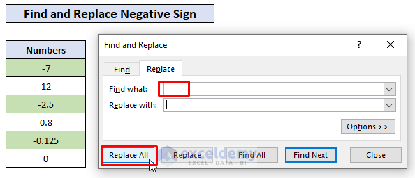
   • Press Ctrl+H to bring up the Find and Replace dialog box.
   • Or, go to the Home tab, click on Find & Select, and then choose Replace.
4. Enter the search criteria:
   • In the “Find what” field, enter a minus sign “-”.
   • Leave the “Replace with” field blank.
5. Click “Replace All”: This action will replace all instances of a minus sign with nothing, effectively turning negative numbers into positive ones.
6. Confirm the result: Check your data to ensure all negative numbers have been converted.

🔍 Note: This method will not remove the numbers themselves, only the negative sign, leaving you with the absolute values of your data.

Using Excel Formulas

If you need to keep the original data intact but want to display only positive numbers, you can use Excel formulas:

• MAX function:

  Formula	Explanation
  =MAX(A1, 0)	This will display the value of cell A1 if it’s positive; otherwise, it will show 0.

  
  
• IF function:

  Formula	Explanation
  =IF(A1<0, "", A1)	This formula will only show the cell value if it’s greater than or equal to 0, otherwise, it will leave the cell blank.

• ABS function:

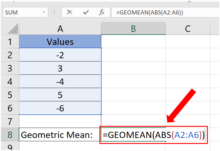
  Formula	Explanation
  =ABS(A1)	This function returns the absolute value of the number in cell A1, effectively making all numbers positive.

Conditional Formatting

If you simply want to hide or highlight negative numbers without altering the data itself:

1. Select the range: Choose the cells you want to apply this conditional formatting to.
2. Go to Home > Conditional Formatting:
3. Choose “New Rule”:
   • Select “Use a formula to determine which cells to format.”
   • Enter the formula =A1<0, assuming A1 is the first cell in your selected range.
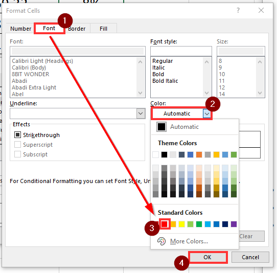
4. Set the Format: Choose how you want negative numbers to appear, like changing their font color to match the background or turning the text white to effectively hide it.
5. Click “OK” to apply: Now, negative numbers will be formatted in a way that makes them less prominent or invisible.

🌟 Note: This method does not delete the negative numbers but merely changes how they are displayed, which can be useful for data visualization or when you need to focus on positive values.

Using Excel Power Query

For larger datasets or for a more automated approach, you can use Excel’s Power Query to remove negative numbers:

1. Select your data range: Highlight the data you want to clean.
2. Go to Data > From Table/Range: This loads your data into Power Query.
3. Choose “Remove Rows”:
   • In the Power Query Editor, click on the column where you want to remove negative values.
   • From the “Home” tab, select “Remove Rows” > “Remove Bottom Rows” and enter 0 in the dialog box, then click “OK”.
4. Close and Load: Once you’ve set up your query, you can close and load the data back into Excel, minus the negative numbers.

🛠️ Note: Power Query provides a powerful way to manipulate data before it's even imported into your workbook, making it an excellent choice for data cleaning tasks.

In summarizing these methods, Excel offers multiple approaches to handle negative numbers, from simple adjustments to more complex data transformations. You can choose the method that best fits your specific needs, whether it’s immediate data manipulation or maintaining an original dataset while altering how the data is presented. Each technique has its own merits, ensuring that no matter the complexity of your spreadsheet or your familiarity with Excel, you’ll find a solution that meets your requirements.

Why would I need to remove negative numbers from my data?

+

Removing or handling negative numbers might be necessary for various reasons like focusing only on positive outcomes, financial reporting where deficits are not required, or performing calculations that exclude negative values.

Will using Find and Replace change my original data?

+

Yes, the Find and Replace method directly modifies the data in your spreadsheet, converting negative numbers to their positive counterparts. Always ensure you have a backup if you need to preserve the original data.

Can I automate the removal of negative numbers in Excel?

+

Yes, Excel’s Power Query is an excellent tool for automating data cleaning tasks, including removing negative numbers, especially for large datasets or recurring tasks.