5 Simple Steps to Delete Blank Rows in Excel Quickly

Are you staring at an Excel spreadsheet filled with data, but also cluttered with blank rows? Blank rows might seem insignificant at first glance, but they can wreak havoc on data analysis, sorting, and overall productivity. Removing these rows can not only clean up your spreadsheet but also enhance its performance. Let's dive into a comprehensive guide on how to delete blank rows in Excel quickly using five simple steps, ensuring your data stays organized and manageable.
Step 1: Prepare Your Worksheet

- Save a Backup: Before you proceed with any data manipulation, always save a backup of your original file. This prevents data loss if something goes awry.
- Check for Hidden Data: Make sure there are no hidden rows or columns where data might be hiding. Use the keyboard shortcut Ctrl+A to select all, then check for any hidden areas.
Step 2: Use Excel’s Filter Feature

- Highlight All Cells: Press Ctrl+A to select your entire worksheet or select the range of cells you want to clean up.
- Apply the Filter: Navigate to the Data tab on the ribbon, then click Filter. Small arrows will appear in each column header.
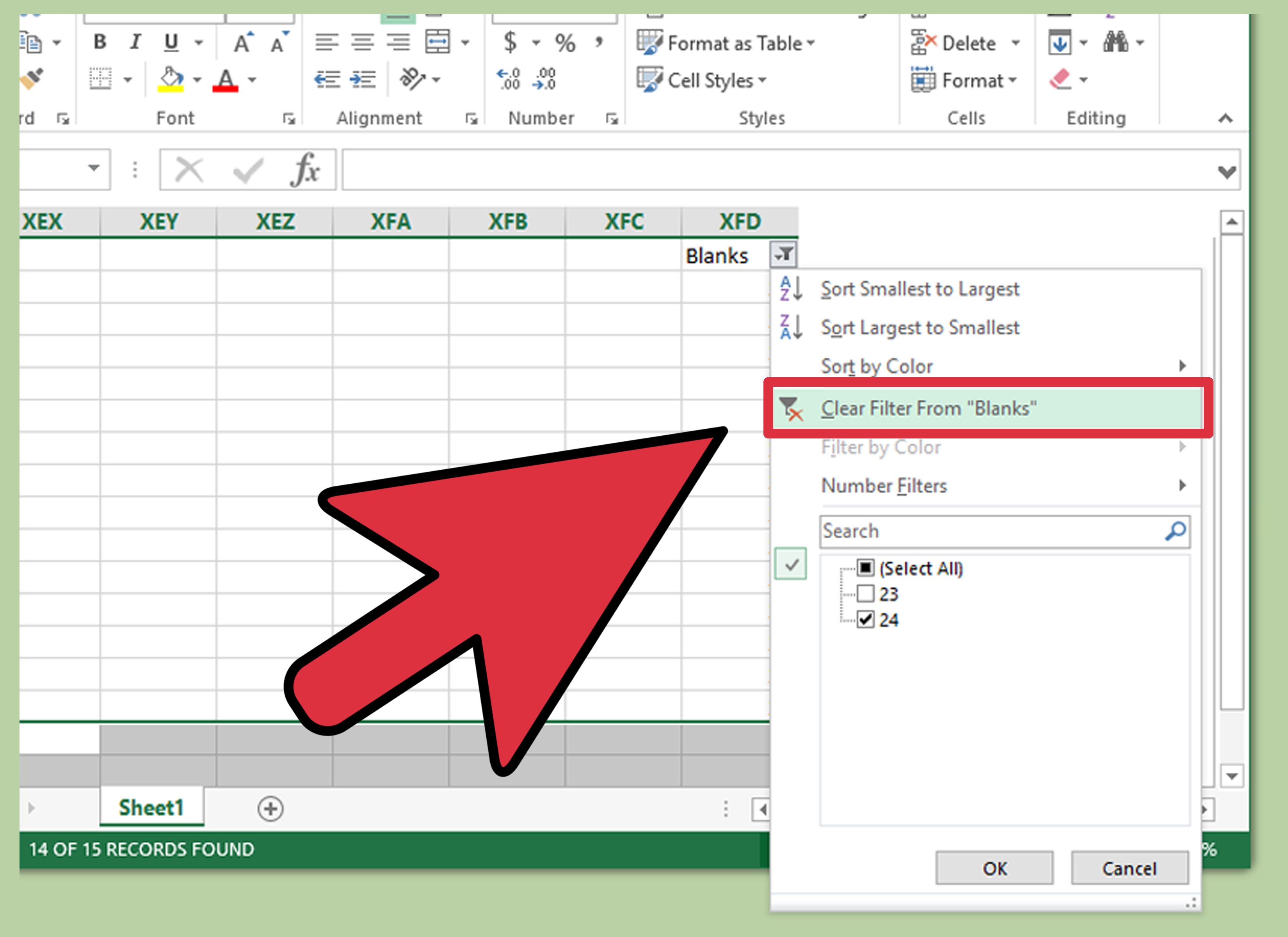
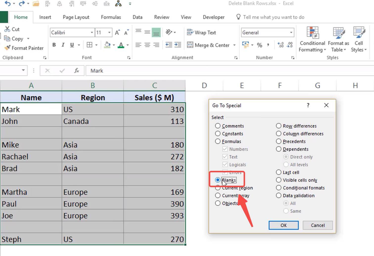
- Filter Blank Rows: Click the arrow in any column header with potential blank cells. Uncheck Select All, then check Blanks to only show rows with empty cells.
Step 3: Select and Delete the Blank Rows

- Highlight All Blank Rows: With the filter in place, all blank rows are now visible. Select the row numbers on the left side of the spreadsheet where the blank rows appear.
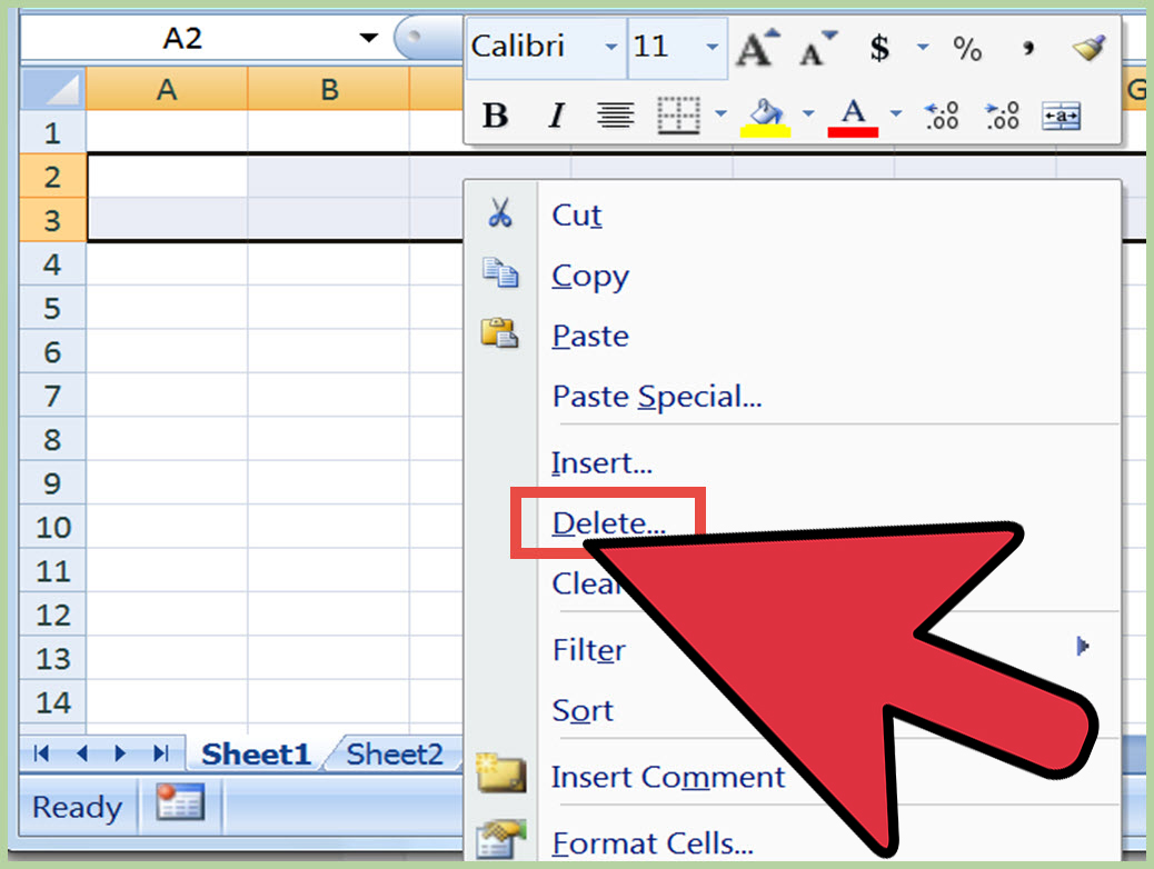
- Remove Rows: Right-click on any of the selected row numbers and choose Delete Row. Excel will delete all highlighted blank rows simultaneously.
🧐 Note: If you're dealing with a large dataset, the process might take a moment. Be patient, and ensure you don't interrupt the process.
Step 4: Reset Filters and Remove Blank Columns

- Clear Filters: Go back to the Data tab and click Filter to clear the filters, returning your worksheet to its original state minus the blank rows.
- Remove Blank Columns: If blank columns remain, repeat the filtering process for columns this time, selecting Blanks and deleting the columns as you did with rows.
Step 5: Final Cleanup and Verification

- Check for Remaining Blanks: Once you’ve removed all visible blank rows and columns, perform a final check using the find-and-replace tool (Ctrl+F) with “find what” set to a blank space to catch any remaining empty cells.
- Save and Review: After deleting blank rows, save your file and review to ensure no essential data was inadvertently removed.
This straightforward approach to cleaning your Excel data not only helps in maintaining a lean and efficient spreadsheet but also significantly boosts your productivity when working with large datasets. By utilizing Excel's filtering features, you're able to effectively pinpoint and remove blank rows with precision, ensuring data accuracy and optimal worksheet performance.
Can this method also work for blank columns?

+
Yes, the method outlined above can be used to delete blank columns by filtering for blanks in column headers instead of row numbers.
What if I accidentally delete rows with important data?

+
Always save a backup before starting the deletion process. If you’ve accidentally deleted rows, you can recover your original data from the backup or use Excel’s undo feature (Ctrl+Z) immediately after the mistake.
Is there a way to automate this process in Excel?

+
Yes, you can automate this process using VBA (Visual Basic for Applications). By writing a macro, you can script Excel to identify and remove blank rows or columns automatically.