5 Easy Steps to Refresh Your Excel Pivot Table

Microsoft Excel's Pivot Table feature is incredibly useful for summarizing, analyzing, and presenting data in a digestible format. Whether you're dealing with large datasets or need quick insights, pivot tables can streamline your work. Over time, however, your pivot table might need a refresh to reflect changes in the underlying data or to adjust its settings for better insights. Here are five straightforward steps to refresh your Excel Pivot Table, ensuring your data analysis is up-to-date and efficient:
Step 1: Refreshing the Data Source

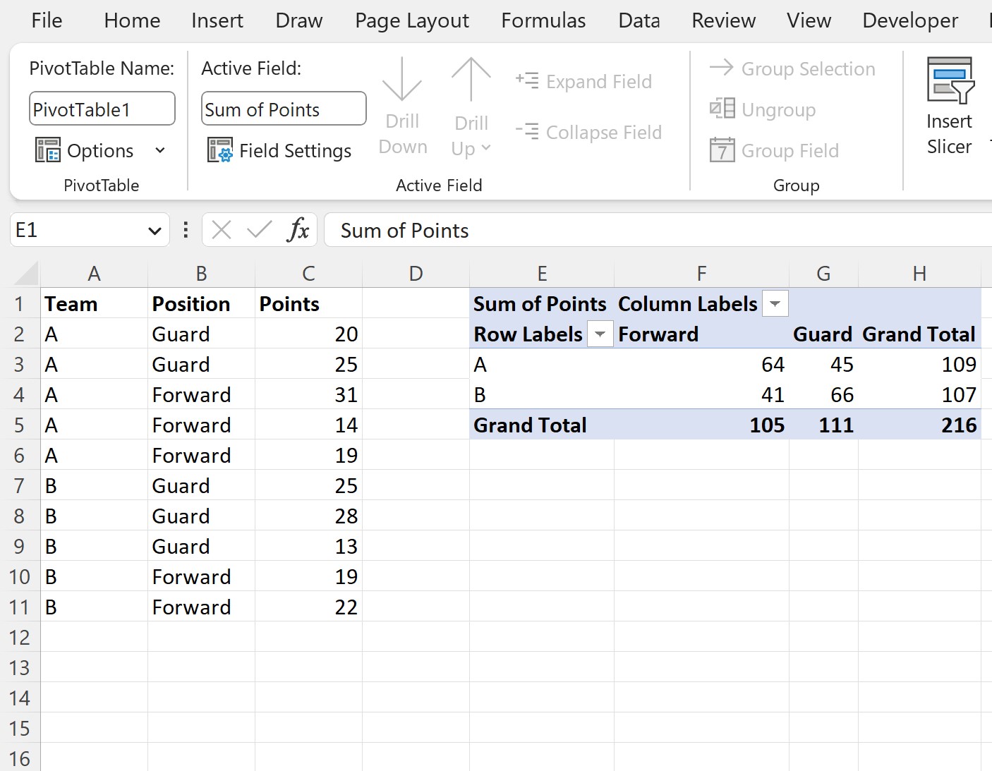
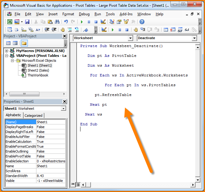
When the data in your source table changes, your pivot table won’t automatically update to reflect these changes. Here’s how you can manually refresh your pivot table:
- Select any cell within the pivot table.
- Go to the PivotTable Analyze tab on the Ribbon.
- Click on the Refresh button, or press Alt + F5 for a keyboard shortcut.
Alternatively, right-click on any cell in the pivot table and choose 'Refresh' from the context menu. If your workbook has external data connections, you might need to:
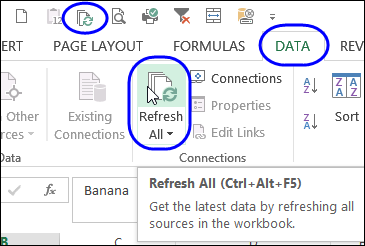
- Navigate to the Data tab.
- Click Refresh All to update all data connections in your workbook.
📝 Note: If you're dealing with an external data source, make sure your data connection is still valid before attempting to refresh.
Step 2: Changing the Data Source

When your original dataset changes size or location, you’ll need to adjust your pivot table’s data source:
- Select any cell in the pivot table.
- Go to PivotTable Analyze > Change Data Source.
- In the dialog box that appears, either type or select the new range for your pivot table data.
📝 Note: If you've added columns to your data, remember to adjust the column letters in your range to include these new fields.
Step 3: Updating the Fields and Layout

Adding new fields or changing how you view your data might require altering the pivot table layout:
- Click on the Field List (usually found next to the pivot table or in the Ribbon under ‘Field List’).
- Drag fields to the appropriate areas: Report Filter, Column Labels, Row Labels, or Values.
- If you’ve added new fields to your data source, they’ll appear under the Fields section. Drag these into the layout as needed.
Here's how the field layout might look:
| Area | Purpose |
|---|---|
| Report Filter | Filter entire pivot table by specific criteria. |
| Column Labels | Create column headers for your analysis. |
| Row Labels | Provide row headers for vertical comparison. |
| Values | Data to be summarized, such as sums, counts, or averages. |

Step 4: Updating Styles and Formats

Not only does your pivot table need to reflect accurate data, but it should also look visually appealing:
- Go to PivotTable Analyze > PivotTable Styles to choose from preset styles.
- To format numbers or dates, right-click a cell in the pivot table, choose Number Format, and select your desired formatting options.
- To group dates or numbers:
- Select the cells containing your dates or numbers.
- Right-click and choose Group… from the context menu.
- Set the grouping interval as required.
📝 Note: Pivot table styles allow for quick aesthetic updates, but remember that the underlying data's presentation remains the core focus.
Step 5: Saving and Preserving Settings

After all your adjustments, you’ll want to save your pivot table’s new settings for future use:
- Right-click the pivot table, then select PivotTable Options.
- In the Layout & Format tab, you can choose to preserve formatting or update on refresh.
- Consider saving your pivot table layout as a template:
- Go to File > Options > Save.
- Click on Default Personal Templates and select the folder where you want to save your template.
Remember, these settings will apply to all future pivot tables unless you change them again.
By following these five steps, you'll ensure your Excel Pivot Table remains an effective tool for data analysis. Whether you're refreshing data, updating the source, tweaking the layout, improving visual aesthetics, or saving settings for consistent use, these steps keep your pivot table up-to-date and efficient. Regular maintenance of your pivot table means your analysis will always be at its best, providing accurate and useful insights for decision-making and reporting.
Why doesn’t my pivot table automatically update?

+
Excel pivot tables typically do not auto-update because changes in the source data can impact the overall structure of the pivot table. To ensure accuracy and consistency, you need to manually refresh the pivot table after modifying the data or adjusting your connection settings.
Can I customize my pivot table refresh settings?

+
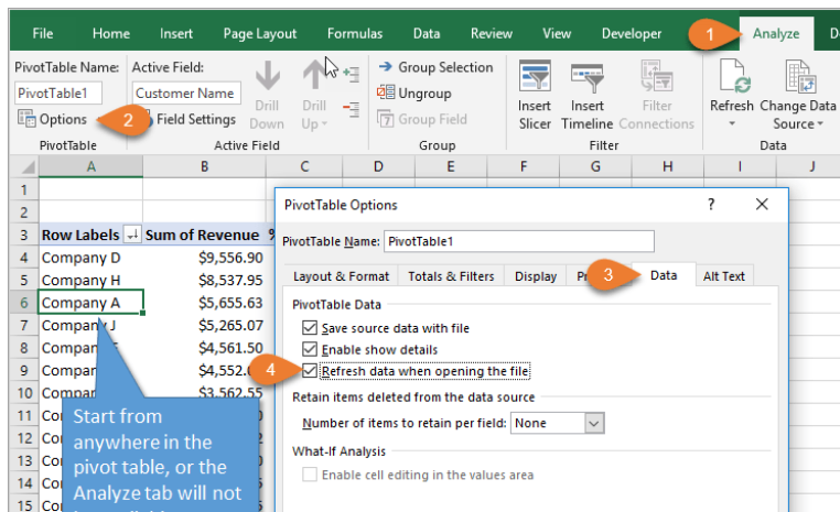
Yes, you can customize the refresh behavior in Excel. Go to PivotTable Options, navigate to the Data tab, and there you can choose to refresh when opening the file, to clear old items from filters or dropdowns, and more.
How do I connect to an external data source for my pivot table?

+
Navigate to the Data tab, select “Get Data” or “From Other Sources,” and follow the prompts to connect to your external database or service. Ensure your connection details are correct and the data is accessible. After setting up the connection, refresh your pivot table to pull in the external data.