Pivoting Two Excel Sheets: Simple Steps

Mastering Excel is a vital skill in today's data-driven workplace. One of the more advanced but essential tasks is pivoting two Excel sheets. This technique allows you to merge and analyze data from two different sheets, which is particularly useful in scenarios involving large datasets from multiple sources. Here's how you can pivot two Excel sheets effectively.
Understanding Pivot Tables

Before diving into pivoting two sheets, understanding pivot tables is crucial. A pivot table is an interactive table that automatically aggregates, or groups, data from one or more worksheets. Here’s a brief overview:
- Pivot tables summarize, sort, reorganize, group, count, and total or average data stored in one table or spreadsheet.
- They are dynamic and can be updated as the underlying data changes.
Preparing Your Data

The first step in pivoting two Excel sheets is ensuring your data is well-prepared:
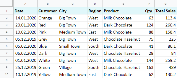
- Ensure Column Headers: Both sheets should have matching headers for the columns you plan to merge. If not, you’ll need to adjust them.
- Remove Blanks: Pivot tables can be thrown off by blank cells, so remove or fill any empty cells with relevant data or zeros.
- Data Consistency: Check for data consistency, like formatting and date types, to avoid mismatches during merging.

Merging Sheets into One Workbook

Before you can create a pivot table from two sheets, these sheets should be within the same workbook:
- Open both Excel workbooks.
- Copy the second sheet: Right-click the sheet tab in the second workbook and choose ‘Move or Copy.’
- Select the destination workbook: From the dropdown, choose the workbook where your first sheet exists.
- Click OK to copy: The sheet will be copied to the new workbook.
Creating a Pivot Table from Two Sheets

Now that your data is in one workbook, follow these steps:
- Select a Cell: In the workbook where you’ve merged both sheets, select any cell in one of the sheets.
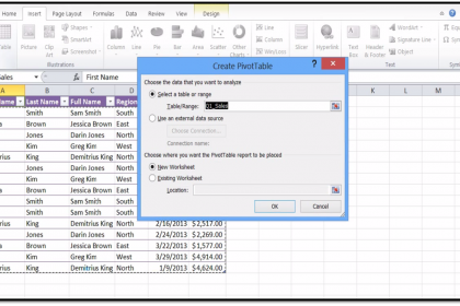
- Insert Pivot Table: Go to Insert > PivotTable to bring up the Create PivotTable dialog box.
- Choose Data Source: Here, you need to combine the data from both sheets:
- Click Multiple consolidation ranges.
- Click Next.
- Consolidate Data: Choose Range List and click Add. Select the range from the first sheet and then repeat for the second sheet.
- PivotTable Fields: Now in the PivotTable Fields pane, drag fields to the Rows, Columns, Values, and Filters areas as needed.
🔍 Note: If your sheets have different ranges or structures, ensure that the data you select covers all relevant rows and columns for accurate consolidation.
Analyzing the Merged Data

With your pivot table set up, here’s how to analyze the merged data:
- Sort: Use the sort options to organize data as needed.
- Filter: Apply filters to narrow down the data you want to view or analyze.
- Summarize with Functions: Use different functions like Sum, Count, Average, etc., to summarize your data.
| Function | Usage |
|---|---|
| Sum | Add up the values for numerical data |
| Count | Count the number of entries |
| Average | Compute the average value |

Tips for Advanced Pivoting

Here are some tips to enhance your pivot table experience:
- Use Calculated Fields: Add custom calculations within your pivot table for complex data analysis.
- Slicers: Use slicers to create visually appealing filters for your pivot table.
- Group Data: Group data to summarize at different levels like dates, numbers, or text.
In summary, pivoting two Excel sheets involves preparation, merging data into one workbook, and effectively using pivot tables to analyze the combined dataset. This skill opens up numerous possibilities for data analysis and decision-making, empowering users to handle complex data scenarios with ease. Remember, mastering Excel tools like pivot tables not only increases efficiency but also provides deeper insights into your data.
Can I pivot more than two sheets in Excel?

+
Yes, you can pivot more than two sheets by following the same process for each additional sheet. Ensure all sheets are in the same workbook, then consolidate them into the pivot table.
What if my data has no common headers between sheets?

+
If headers do not match, you might need to manually adjust them or use Excel functions like VLOOKUP or INDEX-MATCH to align the data before creating the pivot table.
How can I refresh data in the pivot table?

+
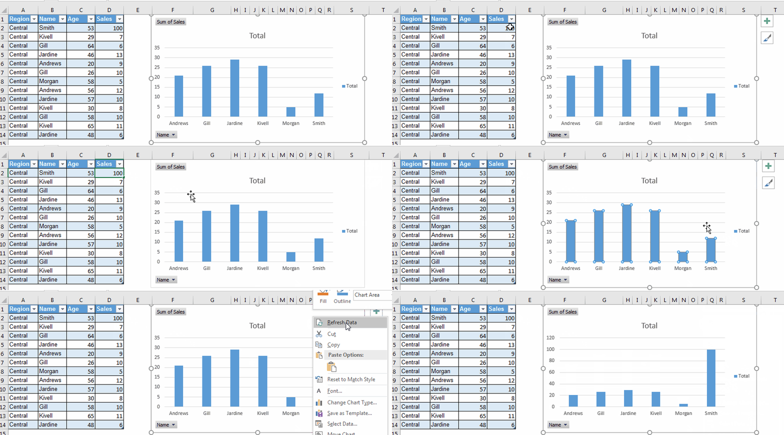
To refresh data, right-click anywhere in the pivot table, go to ‘Refresh’, or use the ‘Refresh All’ button in the Data tab to update all pivot tables in the workbook.