Mastering Excel VLOOKUP with Sheet Naming Tips

Microsoft Excel is a powerful tool that can streamline many aspects of data management and analysis. Among its myriad functions, VLOOKUP is one of the most widely used for finding and retrieving data across different sheets. However, mastering VLOOKUP becomes significantly easier once you understand how to use sheet names effectively. This post will delve into the intricacies of VLOOKUP, explore how to reference sheet names in your formulas, and provide practical tips to enhance your Excel efficiency.
Understanding VLOOKUP

Before we dive into the specifics of sheet names, let’s clarify what VLOOKUP does:
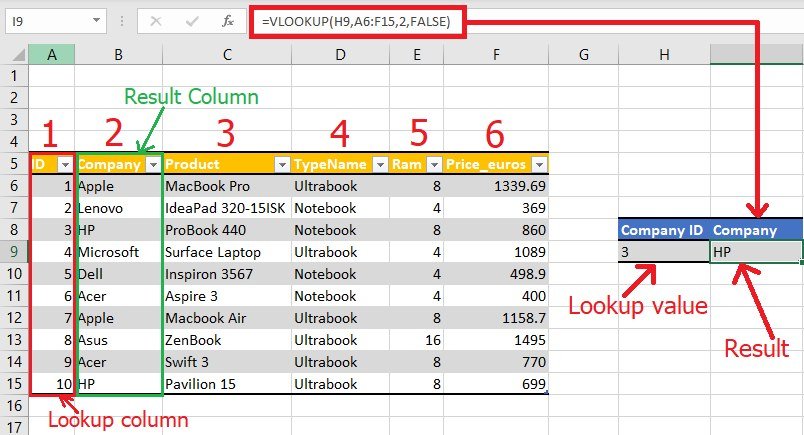
- It vertically looks up for a value in the first column of a table or range.
- It then retrieves a value from the same row in a specified column.
The general syntax of VLOOKUP is:
=VLOOKUP(lookup_value, table_array, col_index_num, [range_lookup])
Components of VLOOKUP:

- lookup_value: The value you want to look up.
- table_array: The range where the lookup_value is searched. This includes the column(s) you want to retrieve data from.
- col_index_num: The column number in the table_array from which to retrieve the value.
- [range_lookup]: An optional argument to specify if you want an exact or approximate match.
Sheet Naming Conventions in Excel

When you’re working with multiple sheets, naming conventions are crucial for clarity and ease of navigation. Here are some tips for effective sheet naming:
- Keep names short and descriptive. For example, “Sales2021” instead of “Annual Sales Figures for the Year 2021”.
- Use underscores or hyphens if necessary: “Sales_Jan” or “Sales-Jan” can help in sorting.
- Avoid spaces. Use CamelCase (“SalesJan”) or underscores to make names more Excel-friendly.
- Maintain consistency across sheets. If you’re naming by date, all sheets should follow the same format.
Referencing Sheet Names in VLOOKUP

Here’s how you reference a sheet name in VLOOKUP:
=VLOOKUP(A2,SheetName!A1:B10,2,FALSE)
This formula looks for the value in A2 on the sheet named "SheetName", then retrieves data from the second column (B) of the range A1:B10.
Using Dynamic Sheet References

To make your formulas more versatile, you can use functions like INDIRECT to dynamically refer to sheet names:
=VLOOKUP(A2,INDIRECT(“‘”&SheetNames!A1&“’!A1:B10”),2,FALSE)
Here, SheetNames!A1 could contain a dynamic sheet name, and INDIRECT will convert this into a proper reference:
🔗 Note: Make sure the cell reference in A1 of SheetNames contains the exact sheet name, including any spaces or special characters enclosed in single quotes if necessary.
Tips for Effective VLOOKUP with Sheet Names

- Check Sheet Names: Always verify the exact spelling and syntax of sheet names to avoid errors.
- Use Defined Names: Define names for cell ranges to make your formulas cleaner and easier to understand. For example:
=VLOOKUP(A2,‘Sales Data’!SalesTable,2,FALSE) - Consistent Naming: Use consistent naming conventions across your workbook to avoid confusion.
- Error Handling: Incorporate IFERROR to handle cases where VLOOKUP might fail:
=IFERROR(VLOOKUP(A2,SheetName!A1:B10,2,FALSE),“Not Found”) - Table References: Use structured references with tables for more intuitive formulas:
=VLOOKUP(A2,[@SalesData],2,FALSE)
Example Scenario

Suppose you have a workbook tracking sales data with separate sheets for each month:
| Sheet Name | Data Range |
|---|---|
| JanSales | A1:D200 |
| FebSales | A1:D200 |
| MarSales | A1:D200 |

If you want to look up sales for a particular SKU (stored in A2) across all sheets, your VLOOKUP formula would change dynamically as follows:
=VLOOKUP(A2,INDIRECT(“‘”&B1&“’!A1:D200”),4,FALSE)
Where B1 contains the current month’s sheet name.
Summing up, VLOOKUP, when combined with effective sheet naming strategies, becomes an exceptionally powerful tool for managing and analyzing data in Excel. By mastering the art of referencing and naming sheets, you can improve your workflow efficiency, ensure data integrity, and create more flexible Excel models. Remember, the key to success in Excel lies not just in knowing the formulas, but in understanding how to make them work together seamlessly.
What if the VLOOKUP function returns #N/A?

+
The #N/A error in VLOOKUP typically means the lookup_value is not found in the first column of your table_array. Ensure the value exists or use IFERROR to handle errors.
How can I reference a dynamic sheet name in Excel?

+
Use the INDIRECT function to create dynamic sheet references. For example: =VLOOKUP(A2,INDIRECT(“‘”&SheetName!A1&“’!A1:B10”),2,FALSE) where A1 of SheetName contains the actual sheet name.
Can I use VLOOKUP across multiple workbooks?

+
Yes, you can. Use the full path to the workbook in the table_array argument like this: =VLOOKUP(A2,‘[WorkbookPath]SheetName’!A1:B10,2,FALSE). However, ensure both workbooks are open when you run this formula.