5 Ways to Match Excel Sheet Columns Easily

Whether you're managing large datasets, analyzing financial records, or organizing an inventory, matching columns in Excel can streamline your workflow. This process can be particularly useful when you're dealing with disparate data sources that need to be integrated or when you want to cross-reference information. Here, we'll explore five effective methods to match Excel sheet columns easily.

Method 1: Using VLOOKUP

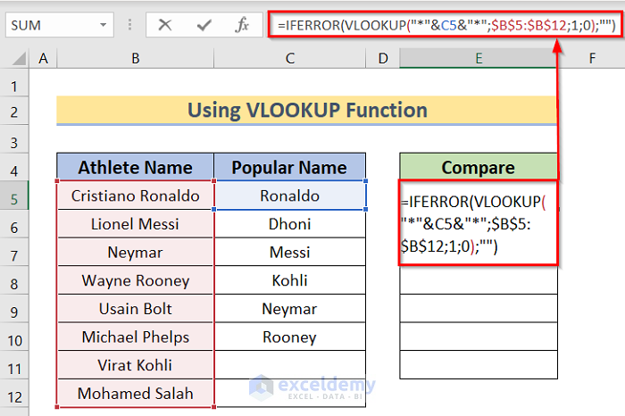
VLOOKUP is one of the most common functions in Excel for matching data between two columns. Here’s how to use it:

• Select a Cell: Click on the cell where you want the matched data to appear.
• Enter the Function: Type =VLOOKUP(lookup_value, table_array, col_index_num, [range_lookup]).
• lookup_value: The value you’re looking for.
• table_array: The range containing the lookup_value and the return value.
• col_index_num: The column number in table_array from which the matching value should be returned.
• [range_lookup]: Use TRUE for approximate match or FALSE for an exact match.
• Adjust as Necessary: Drag the formula down to fill the column or adjust the range to match the entire dataset.

📌 Note: Remember that VLOOKUP requires the lookup column to be on the leftmost side of the lookup table array. If your column to match is on the right, you might need to reorganize your data or consider other methods like INDEX-MATCH.

Method 2: INDEX-MATCH

When flexibility is key, INDEX-MATCH offers more control than VLOOKUP:

• INDEX Function: This function returns the value of a cell in a table based on the row and column numbers you specify.
• MATCH Function: This function searches for a specified item in a range of cells, and then returns the relative position of that item within the range.
• Combination: Use MATCH to find the row position, then INDEX to retrieve the data from that row. The formula looks like this: =INDEX(return_range, MATCH(lookup_value, lookup_range, 0)).

This method is versatile because MATCH can work with both horizontal and vertical ranges, and you can return data from any column, not just the first one.

Method 3: Using Power Query

Power Query, available in newer versions of Excel, is a powerful tool for merging datasets. Here’s how you can use it to match columns:

• Open Power Query Editor: Go to Data > Get & Transform Data > From Table/Range.
• Merge Queries: Select your two tables, click “Home” tab, and choose “Merge Queries.”
• Select Matching Columns: Choose the columns to match, and decide how they should be merged (Inner, Left Outer, etc.).
• Expand the Merged Column: Click on the double arrows at the top of the merged column to select which columns to bring into the main table.
• Load: After transforming your data, load it back into Excel.

🔍 Note: Power Query provides a visual interface for data manipulation, making it particularly useful for those less comfortable with formulas or when dealing with complex data transformation tasks.

Method 4: Conditional Formatting

This method doesn’t match columns in a traditional sense but uses visual cues to highlight matching entries:

• Select Data: Highlight the column you want to compare.
• Open Conditional Formatting: Go to Home > Conditional Formatting > New Rule.
• Use Formula: Select “Use a formula to determine which cells to format” and use a formula like =COUNTIF(lookup_range, A1)>0</code> where A1 is the cell in the current row of the lookup column.
• Set Formatting: Choose how you want the matched entries to be formatted (e.g., highlight in color).
• Apply: Click OK, and Excel will format the cells that match based on your criteria.

This method helps in quickly spotting matches or mismatches visually, which can be useful in data validation scenarios.

Method 5: Using Macros and VBA

For automation and when you need custom matching logic, VBA can be your go-to:

• Open VBA Editor: Press Alt + F11 or go to Developer > Visual Basic.
• Create a New Module: Right-click on any of the objects in the Project Explorer, choose Insert > Module.
• Write the Code: Here’s a basic example of how you might write a VBA code to match columns:

Sub MatchColumns()
    Dim ws1 As Worksheet, ws2 As Worksheet
    Set ws1 = ThisWorkbook.Sheets(“Sheet1”)
    Set ws2 = ThisWorkbook.Sheets(“Sheet2”)

Dim lastRow As Long
lastRow = ws1.Cells(ws1.Rows.Count, 1).End(xlUp).Row

For i = 2 To lastRow 'Assuming data starts in row 2
    'Lookup value from column A in Sheet1
    Dim lookupValue As Variant
    lookupValue = ws1.Cells(i, 1).Value

    'Find the value in Sheet2
    Dim found As Range
    Set found = ws2.Range("A:A").Find(lookupValue, LookIn:=xlValues, LookAt:=xlWhole)

    If Not found Is Nothing Then
        'Column to match is B
        ws1.Cells(i, 2).Value = found.Offset(0, 1).Value
    End If
Next i


End Sub

• Run the Macro: Go back to Excel, press Alt + F8, select your macro, and run it.

VBA provides the ability to handle complex matching scenarios, custom logic, and can automate repetitive tasks.

Each method has its strengths, and the choice will depend on the size of your dataset, your comfort level with Excel formulas or programming, and the specific requirements of your data analysis task. Here's how each method might suit different scenarios:

• VLOOKUP is simple for beginners but limited in functionality.
• INDEX-MATCH is more flexible for advanced users.
• Power Query is excellent for complex data transformation without much formula knowledge.
• Conditional Formatting serves well for quick visual checks.
• VBA Macros are the choice for those needing custom logic or automation.

By employing these methods, you can enhance your data matching capabilities in Excel, making your work not only more efficient but also less prone to human error. As data management continues to be a critical skill in today's business environment, mastering these techniques will keep you ahead in data analysis and processing.

What’s the difference between VLOOKUP and INDEX-MATCH?

+

VLOOKUP is simpler to use but less flexible, as it requires the lookup column to be the first column in the table array. INDEX-MATCH, while more complex, allows you to look up values from any column and is more adaptable to changes in the dataset structure.

Can I use Power Query on older versions of Excel?

+

Power Query was introduced in Excel 2016. For earlier versions, consider upgrading to a newer version or using add-ons like Power Query for Excel, which could provide similar functionality.

How do I match columns if they are not exactly the same?

+

For inexact matches, consider using functions like FUZZY LOOKUP or incorporate wildcard characters in VLOOKUP or INDEX-MATCH for partial string matching.