5 Simple Ways to Match Columns in Excel

Excel's powerful data manipulation tools allow users to perform complex operations with ease. One of such operations is matching data across columns, which is crucial for data analysis, cleaning, and integration. Here, we'll delve into five straightforward methods to match columns in Excel, enhancing your data management skills.

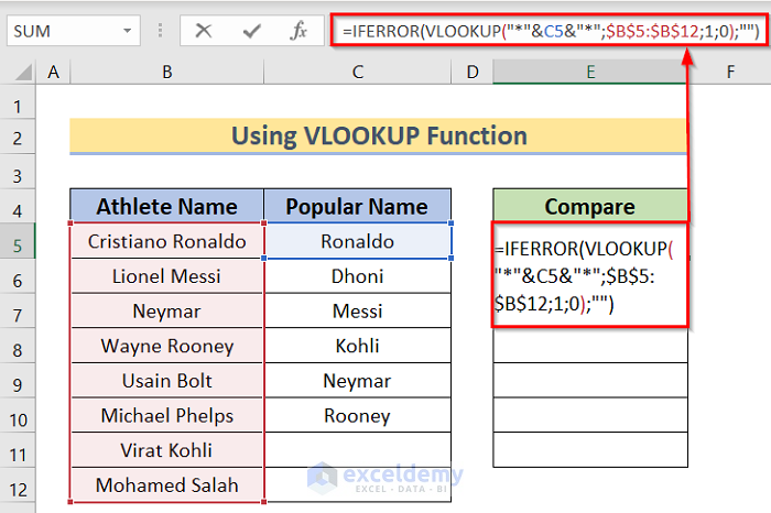
1. Using VLOOKUP for Data Matching

VLOOKUP (Vertical Lookup) is perhaps the most widely recognized function for matching columns in Excel. Here’s how you can use it:

• Identify the column where you want to search for a match (lookup value) and the column from which you want to retrieve data (return column).
• Select the cell where you want to place the result of the VLOOKUP function.
• Enter the following formula: =VLOOKUP(lookup_value, table_array, col_index_num, [range_lookup])
  • lookup_value - The value you are looking up.
  • table_array - The range of cells that contain the lookup and return columns.
  • col_index_num - The column number in table_array from which to retrieve the value.
  • range_lookup - TRUE for an approximate match or FALSE for an exact match.
• Press Enter to see the result.

👀 Note: VLOOKUP will return an #N/A error if no match is found. You can handle this by wrapping the VLOOKUP function with the IFERROR function to manage errors gracefully.

2. Index Match for a More Flexible Lookup

For more control over the lookup direction and when dealing with columns inserted into the lookup table, INDEX MATCH is an excellent alternative:

• MATCH function finds the position of a value in a range: =MATCH(lookup_value, lookup_array, [match_type])
  • lookup_value - The value to match within the lookup array.
  • lookup_array - The range of cells containing possible matches.
  • match_type - 1 for less than, 0 for exact match, or -1 for greater than.
• Once you have the position, use the INDEX function to retrieve the corresponding value: =INDEX(array, row_num, [column_num])

👉 Note: INDEX MATCH can handle row and column matches simultaneously, making it more versatile than VLOOKUP.

3. Exact Match with Conditional Formatting

Conditional Formatting can visually assist in matching columns by highlighting cells where data matches:

• Select the columns or rows you wish to compare.
• Go to Home > Conditional Formatting > New Rule.
• Select "Use a formula to determine which cells to format."
• Enter a formula like =A1=B1 for a simple comparison between adjacent cells or adjust as needed for your data.
• Choose a fill color or other formatting options to highlight matches.
• Apply the rule.

4. Text to Columns for Matching Text

When you need to match string data within cells, splitting text into separate columns can simplify the process:

• Select the column with the data you want to split.
• Navigate to Data > Text to Columns.
• Choose "Delimited" or "Fixed width" based on your data’s structure.
• Specify delimiters or column breaks.
• Select the destination where the split data should appear.
• Now, you can match columns by comparing individual segments of the text.

📌 Note: If your data has multiple delimiters, choose "Advanced" in the Text to Columns wizard to specify all possible separators.

5. Power Query for Advanced Matching

For more complex matching or when dealing with large datasets, Power Query is your go-to tool:

• Select the range of data or open a worksheet with your data.
• Go to Data > Get Data > From Other Sources > Blank Query or From Table/Range.
• In the Power Query Editor, use the Merge Queries option to combine or join data from different tables.
• Specify the matching columns and decide how to merge (Left Outer, Right Outer, etc.).
• Load the merged data back into Excel.

Power Query offers additional functionalities like error handling, data transformation, and step-by-step query editing, which are particularly useful for extensive data matching tasks.

As we wrap up our exploration of matching columns in Excel, it's clear that Excel provides a range of tools tailored to different needs. Whether you need a quick, simple lookup or a sophisticated data integration, these methods can significantly streamline your work. Key takeaways include the use of VLOOKUP for straightforward matching, the versatility of INDEX MATCH, the visual aid of Conditional Formatting, the preprocessing capabilities of Text to Columns, and the advanced matching power of Power Query. Understanding these functions allows you to navigate data with precision and efficiency, ensuring that your datasets are correctly aligned for optimal analysis.

Can I use VLOOKUP to match columns from different sheets?

+

Yes, VLOOKUP can look up data from another sheet. Just reference the sheet name in the table_array argument.

How do I handle errors in INDEX MATCH?

+

You can use the IFERROR function to manage errors gracefully, like =IFERROR(INDEX(array, MATCH(lookup_value, lookup_array, 0)), “No Match”).

What if I need to match only part of a string?

+

Use wildcards within functions like VLOOKUP or MATCH. For example, =VLOOKUP(”” & part_string & “”,…) to match partial strings.