Easily Match Data Across Two Excel Sheets: Simple Guide

When working with data, especially in a business or academic setting, you often need to compare information across multiple Excel sheets. This could be for anything from cross-referencing sales records, synchronizing customer databases, or merging project data. Excel, with its powerful set of tools, simplifies this task through various functions, making data matching both quick and reliable.
Understanding the Basics

Before diving into the how-to, let’s establish why matching data is crucial:
- Data Integrity: Ensure that the information across different spreadsheets remains consistent.
- Error Detection: Identify discrepancies or errors in data entry or updates.
- Reporting: Prepare comprehensive reports by combining and comparing datasets.
Methods to Match Data in Excel

There are several ways to match data in Excel, each with its own use case:
Using VLOOKUP

VLOOKUP is one of Excel’s lookup functions that can easily match data:
- Insert a column where you want the matched data to appear.
- Enter the formula:
=VLOOKUP(lookup_value, table_array, col_index_num, [range_lookup])
- Drag down the formula to fill all cells in the column.
💡 Note: The range_lookup argument determines if you need an exact or approximate match. Use FALSE for exact matches.
Employing INDEX and MATCH

For a more flexible data match, combine INDEX and MATCH:
- Select the cell where you want the result to appear.
- Write the formula:
=INDEX(return_range, MATCH(lookup_value, lookup_range, 0))
- Copy the formula to other cells if needed.
Power Query

Power Query is ideal for more complex data matching tasks:
- Go to the “Data” tab, then “Get Data” > “From File” > “From Workbook.”
- Select the Excel files to merge.
- Use the merge option in Power Query to join tables based on matching columns.
Advanced Tips for Efficient Data Matching

- Data Cleaning: Before matching, ensure your data is clean. Remove duplicates, trim excess spaces, and standardize formats.
- Using Filters and Conditional Formatting: Highlight or filter rows where data matches or differs for visual comparison.
- Macro Scripts: For repetitive tasks, consider using VBA (Visual Basic for Applications) to automate the matching process.
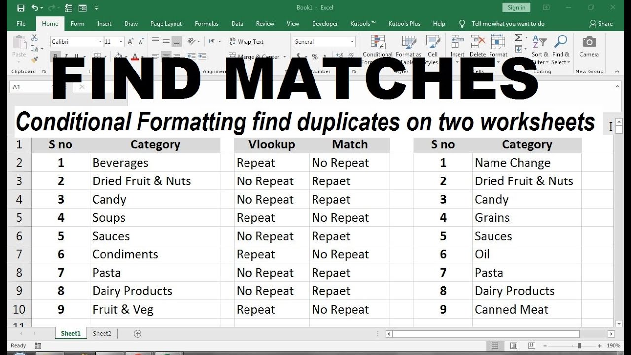
In practice, these methods help you to manage large datasets efficiently. Here is a quick example of how you might set up an Excel table to match data:
| Column A | Column B | Matched Data |
|---|---|---|
| Item Code | Item Name | =VLOOKUP(A2,Sheet2!A:B,2,FALSE) |
| ... | ... | ... |

👉 Note: Always remember to check if the data you are looking up is present in the lookup table to avoid #N/A errors.
Summing up, matching data in Excel can greatly enhance your productivity when managing large datasets. Whether you need to reconcile accounts, consolidate information, or simply check for accuracy, the techniques mentioned provide robust solutions for seamless data integration.
Can I match data from different workbooks using VLOOKUP?

+
Yes, you can use VLOOKUP to match data from different workbooks by referencing the workbook and sheet in the formula:
=VLOOKUP(lookup_value, [WorkbookPath]Sheet!Range, col_index_num, [range_lookup])
How can I handle #N/A errors when matching data?

+
You can wrap VLOOKUP or MATCH functions with IFERROR to return a custom message or an empty cell if no match is found, e.g.,
=IFERROR(VLOOKUP(A2,Sheet2!A:B,2,FALSE),“No Match”)
What should I do if my data contains multiple columns to match?

+
Use Excel’s Power Query to merge multiple columns or concatenate values in a single lookup column. Alternatively, use an array formula with INDEX and MATCH for multi-column matches.