VLOOKUP Mastery: Matching Excel Sheets Easily

Understanding VLOOKUP

In the realm of data management, VLOOKUP stands out as an essential function in Microsoft Excel, designed to assist users in retrieving information across different sheets or tables efficiently. If you’re dealing with large datasets or coordinating between multiple spreadsheets, mastering VLOOKUP can significantly enhance your productivity. This blog post will guide you through the intricacies of VLOOKUP, from basic concepts to advanced techniques, ensuring you can match Excel sheets effortlessly.

The Basics of VLOOKUP

Before diving into the function, let’s understand what VLOOKUP does:

• Vertical Lookup: Searches for a value vertically down the first column of a specified range.
• It then retrieves a value from the same row but in a different column within that range.

Syntax:

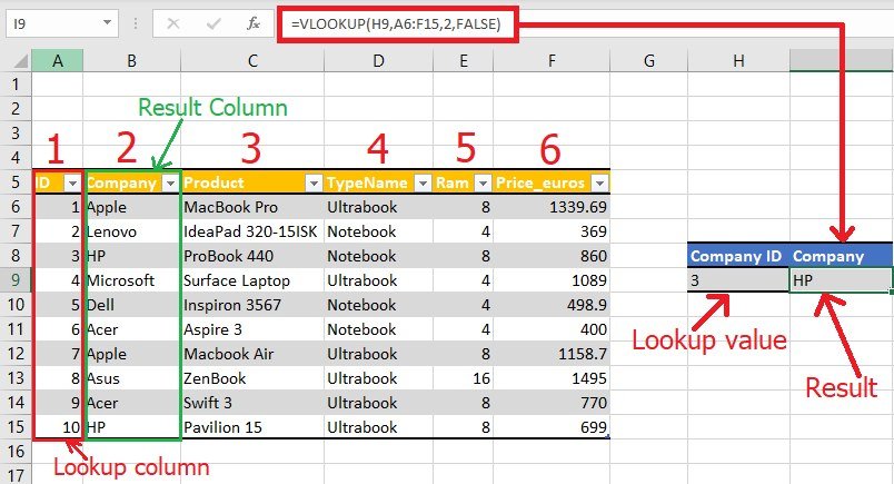
<code>VLOOKUP(lookup_value, table_array, col_index_num, [range_lookup])</code>

Here’s a breakdown:

• lookup_value: The value you’re searching for within the table.
• table_array: The range containing the lookup value and the return value.
• col_index_num: The column number in the table_array from which to retrieve the value.
• [range_lookup] (optional): A logical value specifying whether you want an approximate or exact match. TRUE or 1 for approximate, FALSE or 0 for exact.

Performing a Basic VLOOKUP

To illustrate how VLOOKUP works, imagine you have a sales database with product IDs, names, and prices, and you want to find the price of a specific product:

<table>
  <tr><th>Product ID</th><th>Product Name</th><th>Price</th></tr>
  <tr><td>1</td><td>Laptop</td><td>$1200</td></tr>
  <tr><td>2</td><td>Mouse</td><td>$50</td></tr>
</table>

Here’s how you’d use VLOOKUP:

<code>=VLOOKUP(2, A2:C3, 3, FALSE)</code>

Steps:

• Select the cell where you want the VLOOKUP result to appear.
• Enter the formula as shown above, adjusting the range and column numbers as necessary for your data.
• The formula searches for ‘2’ in column A and returns the value in the third column (Price) of that row.

🔥 Note: Ensure your table_array in the formula includes the column with the lookup_value and the column with the data you want to retrieve.

Advanced VLOOKUP Techniques

Handling Errors with VLOOKUP

Sometimes, VLOOKUP might not find a match, leading to #N/A errors. Here are ways to handle this:

• IFERROR function: Wrap your VLOOKUP in IFERROR to replace errors with a custom message or value:

<code>=IFERROR(VLOOKUP(lookup_value, table_array, col_index_num, FALSE), "Not Found")</code>

• ISNA function: Another approach is using ISNA to check for errors:

<code>=IF(ISNA(VLOOKUP(lookup_value, table_array, col_index_num, FALSE)), "Not Found", VLOOKUP(lookup_value, table_array, col_index_num, FALSE))</code>

VLOOKUP with Approximate Match

If your data is sorted in ascending order, VLOOKUP can find an approximate match:

<code>=VLOOKUP(lookup_value, table_array, col_index_num, TRUE)</code>

This is useful for finding the closest value to your lookup_value, like tax rates or discount levels based on thresholds.

VLOOKUP Limitations and Alternatives

Limitations

• VLOOKUP searches only left to right. It cannot retrieve data from a column to the left of the lookup column unless you rearrange your data or use another function.
• It can be slow with large datasets, affecting performance.

Alternatives

• INDEX and MATCH: This combination is more flexible and can look both left and right:

<code>=INDEX(return_range, MATCH(lookup_value, lookup_range, 0))</code>

• XLOOKUP (Excel 365 and later): A more powerful successor to VLOOKUP, capable of searching vertically or horizontally, returning multiple values, and handling errors more gracefully.

Streamlining Your Workflow with VLOOKUP

Key Tips:

• Name your ranges: This makes your formulas more readable and easier to update if your data changes.
• Use absolute references ($ signs) for cell references in the VLOOKUP formula to prevent errors when copying the formula across cells.
• Sort your data if using approximate matches for better accuracy.
• Consider data validation: Use dropdown lists for lookup values to reduce errors in entry.

To summarize, VLOOKUP is a vital tool for data retrieval in Excel. By mastering it, you can streamline your data management tasks, connect information across spreadsheets, and boost your productivity. From basic lookups to handling errors and dealing with large datasets, VLOOKUP can be tailored to various needs, though knowing its limitations and having alternative methods at hand can further enhance your Excel skills.

How can I make VLOOKUP look up data to the left?

+

By default, VLOOKUP can’t look up data to the left of the lookup column. You can use the INDEX and MATCH functions instead:

=INDEX(return_range, MATCH(lookup_value, lookup_range, 0))

Can VLOOKUP be used with approximate matches?

+

Yes, by setting the fourth argument to TRUE or 1 in the VLOOKUP formula, you allow it to find an approximate match if the data is sorted in ascending order.

What are the best practices for using VLOOKUP efficiently?

+

- Use Named Ranges for better readability.
- Use absolute references to keep the lookup range consistent when copying formulas.
- Ensure your data is sorted if using approximate matches.
- Implement data validation to avoid input errors.