5 Ways to Match Data Across Excel Sheets Easily

Matching data across Excel sheets can seem like a daunting task, but it's actually quite manageable with the right techniques. In this article, we'll delve into five methods that make the process easier and more efficient, enhancing your productivity with Excel. Whether you're a beginner or a seasoned user, these tips will help you streamline your data management tasks.
Using VLOOKUP for Data Matching


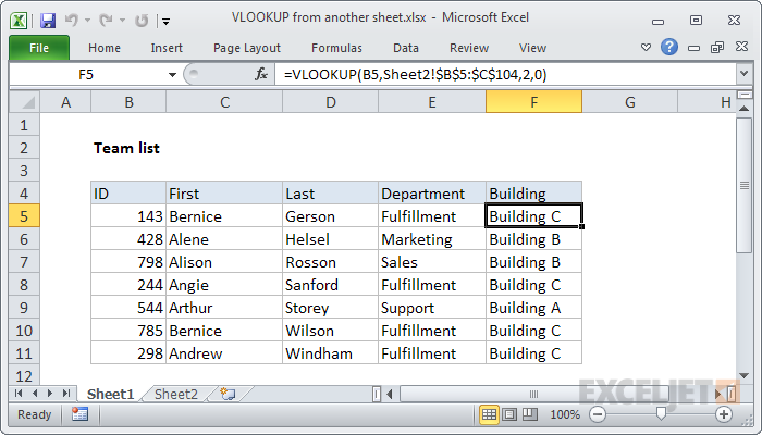
One of the simplest and most common methods for matching data is by using the VLOOKUP function. Here’s how you can utilize it:
- Prepare Your Data: Ensure that the lookup column in the source and destination sheets is exactly the same, including the column header.
- Formula Syntax: Use the formula
=VLOOKUP(lookup_value, table_array, col_index_num, [range_lookup]) - Explanation:
- lookup_value: The value you want to look up.
- table_array: The range of data from which to retrieve the value.
- col_index_num: The column number in the table_array from which to retrieve the value.
- [range_lookup]: TRUE for approximate match or FALSE for an exact match. Typically, for matching data, you would use FALSE.
🔍 Note: VLOOKUP can only look rightward, meaning if your lookup column isn’t the leftmost column in the lookup table, you’ll need to rearrange your data or use INDEX and MATCH.
INDEX and MATCH Function Combination


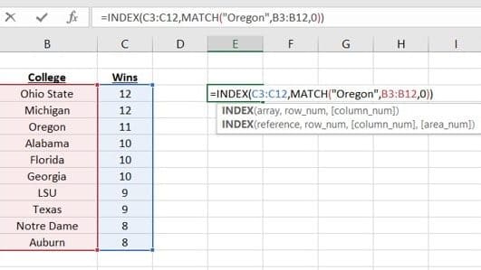
While VLOOKUP is straightforward, INDEX and MATCH provide more flexibility. This combination can look up values in any column, making it superior for some tasks:
- MATCH Function: Use this to find the position of the lookup value within the lookup range.
- INDEX Function: Retrieve the data from the position MATCH has identified.
- Formula Syntax: Use the formula
=INDEX(array, MATCH(lookup_value, lookup_array, match_type)) - Example: If you’re looking to match data based on employee ID, your formula might look like this:
=INDEX(Sheet2!B2:D100, MATCH(A2, Sheet2!A2:A100, 0))
Conditional Formatting for Visual Matching


Conditional formatting provides a visual way to identify matching data:
- Select Range: Choose the range where you want to apply the rule.
- Create Rule: From the Home tab, select Conditional Formatting > New Rule. Choose “Use a formula to determine which cells to format.”
- Formula: Use a formula like
=A2=B2to match values from two columns side by side. - Format: Select a formatting option to highlight matches (e.g., color fill, font style).
🎨 Note: This method is excellent for quick visual checks but not for data manipulation or retrieval.
Pivot Table for Advanced Data Matching


Pivot Tables offer a powerful way to analyze and compare data from different sheets:
- Create a Pivot Table: Go to Insert > Pivot Table and choose your data source.
- Set up your fields: Drag fields to the Rows and Columns areas to analyze and compare.
- Match Data: Use the filter or the Row Label to isolate matching data points.
Power Query for Sophisticated Data Matching


Power Query (part of Excel since 2013) allows for advanced data manipulation, including matching across multiple sheets:
- Launch Power Query: From the Data tab, choose Get & Transform Data, then select Get Data.
- Load Sheets: Import both Excel sheets you want to match.
- Merge Queries: Use the Merge Queries feature to join data based on common columns.
- Expand Data: Once merged, expand the new column to include the matching data.
- Load Back to Excel: Close and Load the query to put the results back into Excel.
In wrapping up, each method has its unique advantages:
- VLOOKUP is perfect for straightforward lookups when the data structure supports it.
- INDEX and MATCH give you more control over where data is pulled from, making it ideal for complex datasets.
- Conditional Formatting offers visual cues which can be invaluable for quick checks.
- Pivot Tables are excellent for multi-dimensional analysis and grouping.
- Power Query stands out for its ability to handle large datasets and intricate data transformation tasks.
By mastering these techniques, you can match data in Excel with greater ease and accuracy. Whether it’s for auditing, data reconciliation, or merging datasets, these methods ensure that you’re equipped to handle any data-matching task efficiently.
This article doesn’t merely provide techniques; it arms you with the tools to make Excel a more powerful ally in your data analysis endeavors. Keep in mind that the best method often depends on the complexity of your data and your specific requirements. Experiment with these techniques to find which one suits your workflow best.
Why does VLOOKUP sometimes return an error?

+
VLOOKUP can return an error if the lookup value is not found, the lookup column is not the leftmost, or if there’s a mismatch in the data type between the lookup value and the table_array. Ensure your data is formatted correctly and consider using exact match (FALSE).
Can I match data between sheets from different Excel files?

+
Yes, using Power Query, you can load data from multiple Excel files into a single query. From there, you can merge and match the data as needed.
What’s the difference between exact and approximate match in VLOOKUP?

+
An exact match (FALSE) requires the lookup value to be exactly present in the first column of the lookup table. An approximate match (TRUE) finds the closest match, which can be useful for sorted ranges where an exact match isn’t necessary.