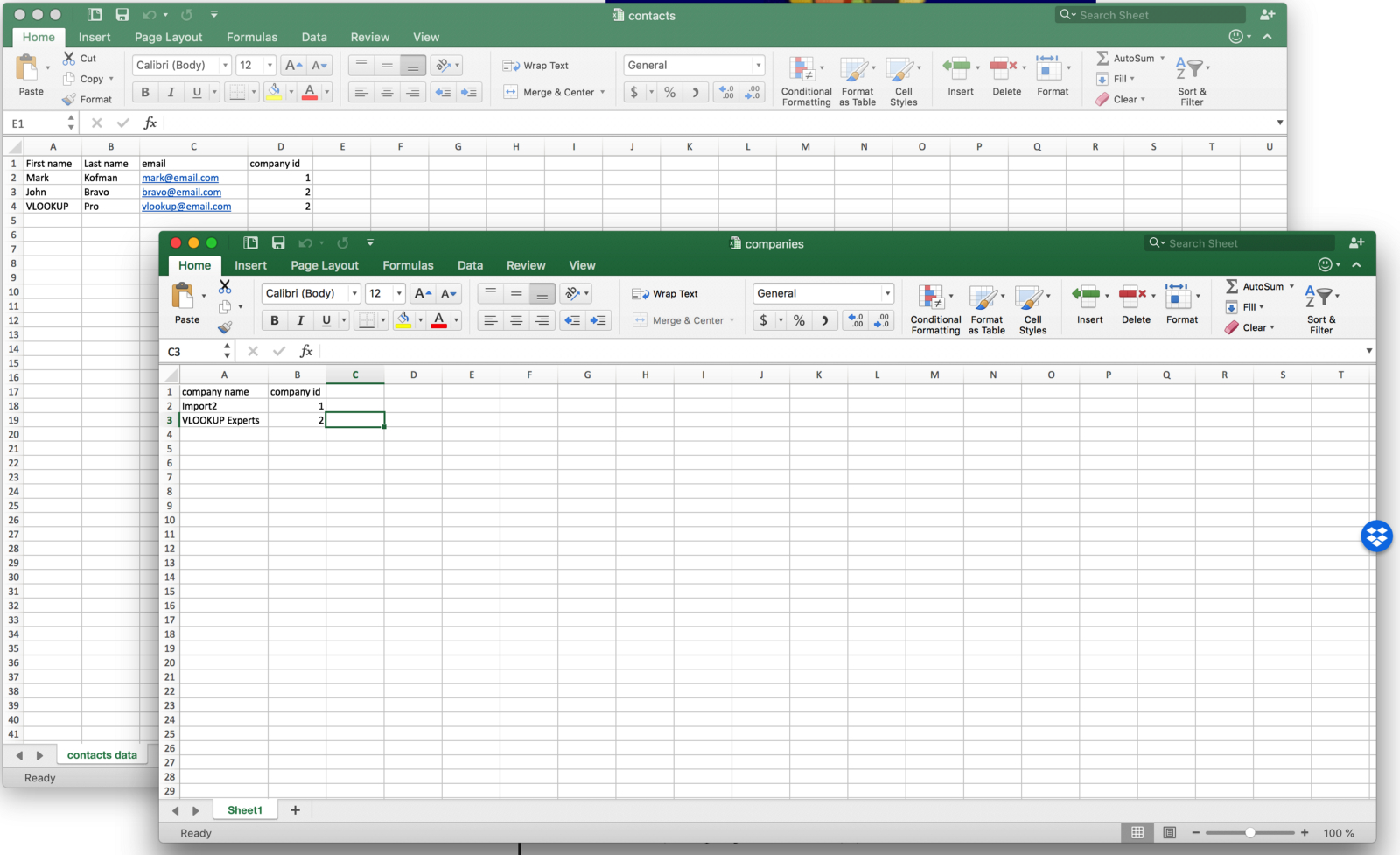
5 Ways to Match Data Between Two Excel Sheets

When dealing with large datasets, ensuring accuracy and consistency is crucial. Excel users often find themselves needing to match data across different spreadsheets. Whether you're reconciling financial reports, comparing lists, or simply cleaning your data, matching data between two Excel sheets can streamline your workflow significantly. This post will explore five effective methods to accomplish this task efficiently.
1. VLOOKUP Function

The VLOOKUP function is perhaps the most straightforward method for matching data in Excel:
- What it does: VLOOKUP searches for a value in the first column of a table and returns a value in the same row from another column.
- How to use it:
- Select the cell where you want the result.
- Enter
=VLOOKUP(lookup_value, table_array, col_index_num, [range_lookup]). - Ensure lookup_value is the value you want to search for.
- Set table_array to the range of columns where the matching data resides.
- Specify col_index_num for which column number to return the data.
- Choose range_lookup as TRUE for approximate match or FALSE for exact match.
🔍 Note: VLOOKUP requires the lookup value to be in the first column of the table array.
2. INDEX and MATCH Combo

When VLOOKUP falls short due to its limitations, the INDEX and MATCH functions come to the rescue:
- Why use INDEX MATCH: This combination provides flexibility in column placement and can match both horizontally and vertically.
- How to use it:
- In a cell, type
=INDEX(range, MATCH(lookup_value, lookup_array, match_type)). - Define the range where you want to retrieve the result.
- Specify lookup_value and lookup_array for the column where the matching should occur.
- match_type can be 0 for an exact match.
- In a cell, type
Here’s a small example:
| Name | Dept |
|---|---|
| John | Sales |
| Jane | HR |

=INDEX(B1:B2, MATCH("Jane", A1:A2, 0))Which would return "HR" since Jane's department is in HR.
3. Conditional Formatting

Conditional formatting can visually highlight matches or mismatches:
- What it does: It changes the appearance of cells based on the rules you define.
- How to set it up:
- Select the range to format.
- Go to Home > Conditional Formatting.
- Select New Rule.
- Choose "Use a formula to determine which cells to format."
- Enter the formula to compare cells. Example:
=A1=B1to highlight if the cells match.
4. Power Query

Power Query (available in Excel 2016 and later versions) provides an advanced method to merge data:
- Why use Power Query: It allows for complex data transformations and merging without altering your source data.
- How to use Power Query:
- Go to Data > Get Data > From Table/Range.
- In the Power Query Editor, choose Home > Merge Queries.
- Select the tables to merge and choose the matching columns.
- Define how the merge should happen (e.g., Left Outer Join, Inner Join).
- Complete the merge and load the result back into Excel.
5. VBA Scripting

For more control or automation, VBA scripting is a powerful solution:
- What it does: Automates repetitive tasks or complex matching criteria through custom coding.
- How to create a VBA script:
- Press Alt + F11 to open the VBA editor.
- Insert a new module (Insert > Module).
- Write a VBA code to compare and match data. Here’s a basic example:
Sub MatchData()
    Dim wb As Workbook
    Dim ws1 As Worksheet, ws2 As Worksheet
    Dim rng1 As Range, rng2 As Range
    Dim found As Range

    Set wb = ThisWorkbook
    Set ws1 = wb.Sheets("Sheet1")
    Set ws2 = wb.Sheets("Sheet2")
    Set rng1 = ws1.Range("A1:A" & ws1.Cells(ws1.Rows.Count, "A").End(xlUp).Row)

    For Each Cell In rng1
        Set found = ws2.Range("A:A").Find(What:=Cell.Value, LookIn:=xlValues, LookAt:=xlWhole)
        If Not found Is Nothing Then
            Cell.Offset(0, 1).Value = found.Offset(0, 1).Value
        Else
            Cell.Offset(0, 1).Value = "No Match"
        End If
    Next Cell
End Sub
This script will loop through a column in Sheet1 and search for matching values in column A of Sheet2, then write the corresponding value from the adjacent column in Sheet2 back to Sheet1.
By implementing these five methods, you can effectively match data across Excel sheets, enhancing your data analysis, reconciliation, and reporting tasks. Each method offers unique advantages depending on your specific needs, data size, and complexity of the matching task. Remember, mastering these techniques can significantly improve your efficiency with Excel, transforming the way you handle data.
What is the fastest way to match data between Excel sheets?

+
Using Power Query is typically the fastest and most efficient method for matching large datasets due to its advanced merging capabilities.
Can VLOOKUP match data from multiple sheets?

+
Yes, by referencing multiple sheets within the table array, VLOOKUP can match data across different sheets, although it can become complex with large datasets.
Is INDEX and MATCH better than VLOOKUP?

+
INDEX and MATCH offer more flexibility and are generally preferred for their ability to look both horizontally and vertically and to work with columns that are not in the first position of a table.