5 Steps to Convert Excel Sheet to Table
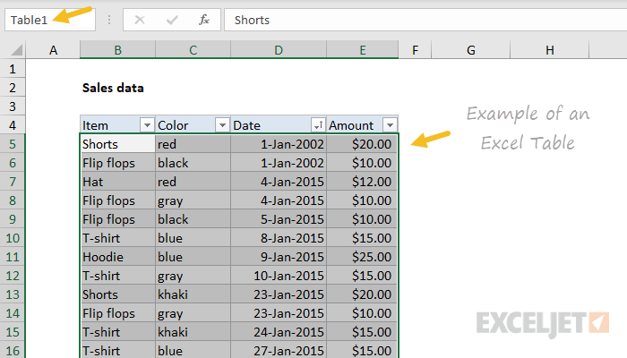
Converting an Excel sheet into a well-formatted table can transform your data into a clear, organized visual that's easy to understand and analyze. Whether you're managing a project, tracking inventory, or presenting data, tables offer a visually appealing and functional way to present information. Here are five comprehensive steps to turn your Excel data into an informative table.
Step 1: Prepare Your Data

Before you can create a table, your data needs to be well-structured:
- Ensure your dataset has headers for each column to clearly define what data each column represents.
- Remove any unnecessary rows or columns to streamline your data presentation.
- Check for and eliminate any duplicate or irrelevant information that might clutter your table.
- Ensure each row represents a unique record or entry.
📝 Note: Consistency in headers and data format improves table functionality.
Step 2: Select Your Data and Insert Table

Now that your data is clean, follow these steps:
- Open your Excel workbook and navigate to the worksheet containing your data.
- Highlight the range of cells you wish to convert into a table.
- Go to the ‘Insert’ tab on the ribbon, and click on ‘Table’.
- In the dialog box that appears, ensure the checkbox for ‘My table has headers’ is ticked if you’ve included headers in your selection.
- Click ‘OK’ to convert your selected range into a table.
| Action | Keyboard Shortcut |
|---|---|
| Select range and insert table | Ctrl + T (Windows) | Cmd + T (Mac) |
Step 3: Customize Your Table
After creating your table, you can customize it to enhance readability and functionality:
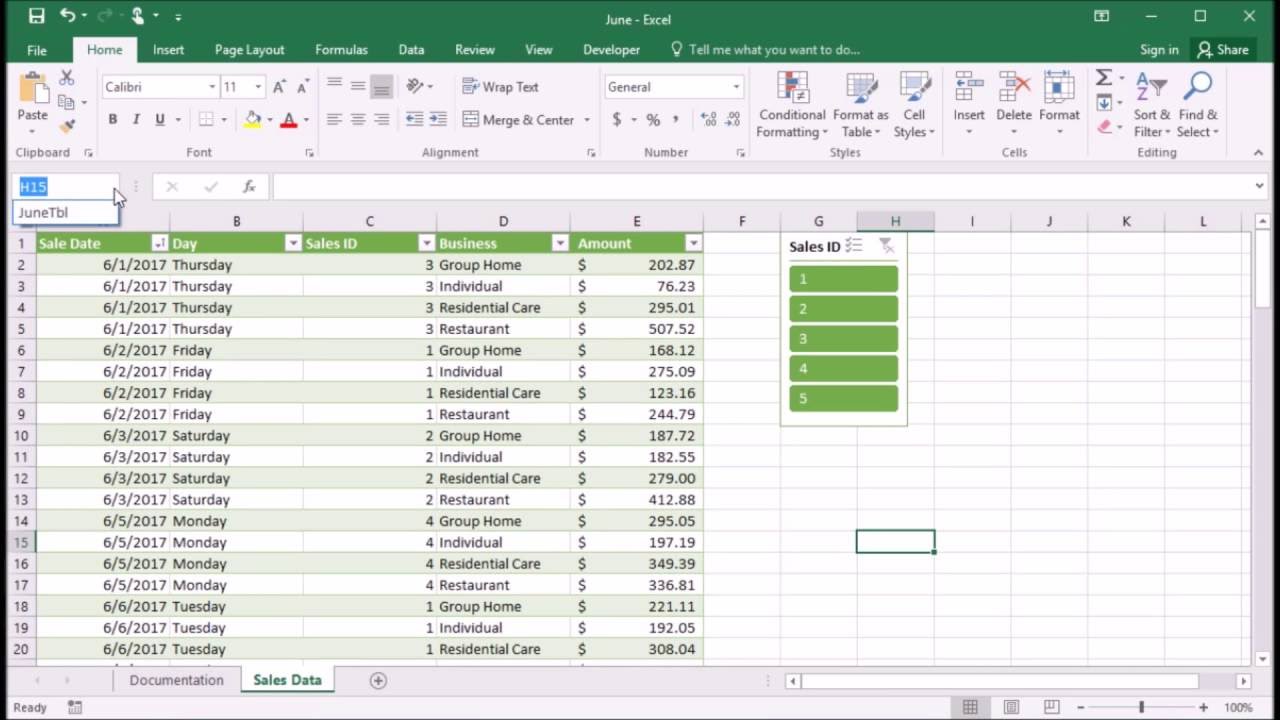
- Style: Choose from various built-in styles in the ‘Table Styles’ section. Adjust the color scheme to match your presentation or corporate branding.
- Format: Apply conditional formatting for better data visualization. For example, highlight cells based on specific criteria like high values or trends.
- Filter: Use the filter dropdowns that appear with the table to sort, filter, or group data as needed.
🎨 Note: Proper styling can significantly enhance the readability and appeal of your data.
Step 4: Handle Totals and Aggregations
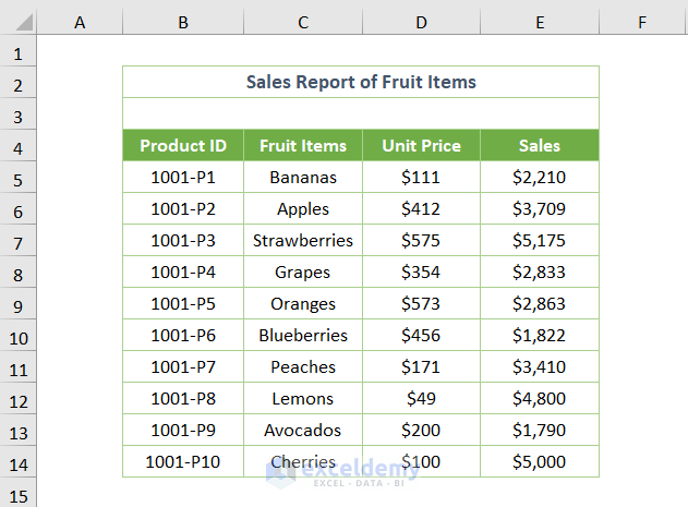
To add summary rows:
- Select any cell within your table.
- Navigate to the ‘Design’ tab under ‘Table Tools’.
- Check the ‘Total Row’ option.
- Select the function you want to apply to each column (sum, average, count, etc.) from the dropdown that appears in the last row of the table.
Step 5: Manage and Expand Your Table

Your table will dynamically expand as you add more data:
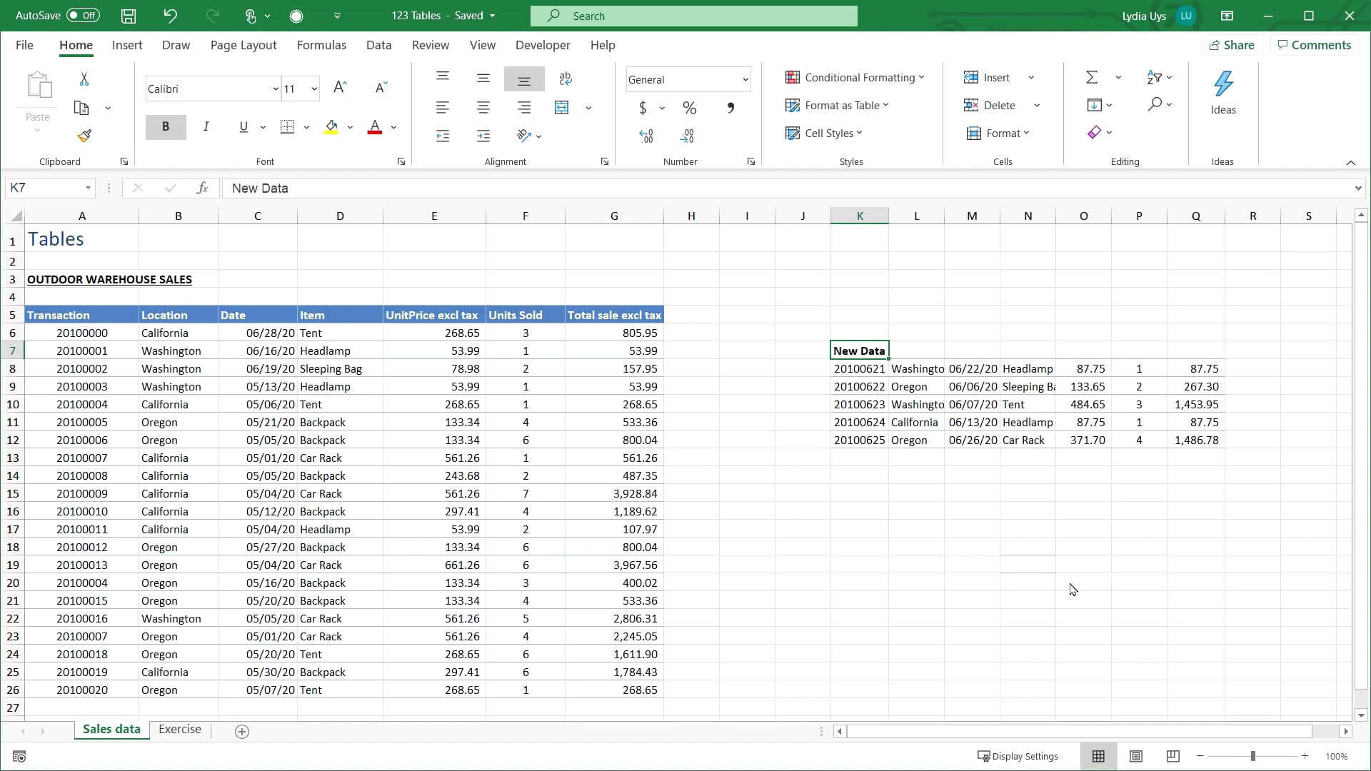
- New rows added will automatically become part of the table if they are within the column range.
- Columns can be resized or added to fit additional data. Simply insert new columns within or next to the table, and they’ll be incorporated.
- To manage the table or revert data, right-click within the table and select ‘Table’ options to access settings like resizing or formatting.
By following these steps, you've not only created a functional table but also made your data more accessible and presentable. This process has equipped you with the tools to efficiently manage your datasets, making analysis and presentations much more straightforward.
Why should I use a table for my Excel data?
+
Using tables in Excel provides numerous benefits like automatic formatting, filters, and easier data management. Tables also make data analysis simpler with tools like sort, filter, and total rows that automatically update as data changes.
Can I convert an existing range into a table?

+
Yes, you can convert any existing range of cells into a table by selecting the range and using the ‘Insert Table’ feature.
How do I add new data to the table?

+
When you add data directly below or beside your table, Excel will prompt you to expand the table, or you can insert new rows/columns within the table’s boundary, and they’ll be included automatically.