5 Easy Ways to Freeze Excel Rows for Better Visibility

Freezing rows in Microsoft Excel is an essential feature for anyone who regularly deals with large datasets. This function allows you to keep specific rows visible while scrolling through the rest of your spreadsheet, enhancing your ability to navigate, analyze, and edit data efficiently. In this post, we'll explore 5 easy ways to freeze rows in Excel, ensuring you can work with better visibility no matter the size of your data.
Why Freeze Rows in Excel?

Before diving into the methods, it's worth understanding why freezing rows can be so advantageous:
- Consistency: Keeps headers or titles in view, ensuring you're always working with the correct data context.
- Efficiency: Reduces the need to scroll back and forth, allowing for quicker data analysis and comparison.
- Visibility: Makes it easier to work with extensive datasets by keeping key rows in place.
1. Freezing the Top Row

Perhaps the most straightforward method, freezing the top row is ideal for datasets where the first row contains headers or titles.
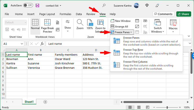
- Select the row below the one you want to freeze. If you want to freeze the top row, simply click into any cell in the second row.
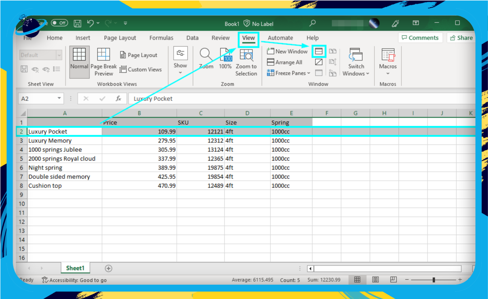
- Go to the "View" tab on the Ribbon.
- In the "Window" group, click on "Freeze Panes".
- Choose "Freeze Top Row" from the dropdown menu.

📌 Note: Excel will freeze all rows above the active cell when you select "Freeze Panes" without choosing a specific option.
2. Freezing Multiple Rows

If your header spans multiple rows, Excel allows you to freeze several at once:
- Select the row below the ones you want to freeze. For example, to freeze the first three rows, click on the fourth row.
- Follow the same steps as freezing the top row, but select “Freeze Panes” instead of “Freeze Top Row”.
💡 Note: The active cell determines where the freeze line is placed; ensure it’s at the right spot before freezing.
3. Freezing Rows and Columns Together

Sometimes, you might want to freeze both rows and columns to create a fixed reference area:
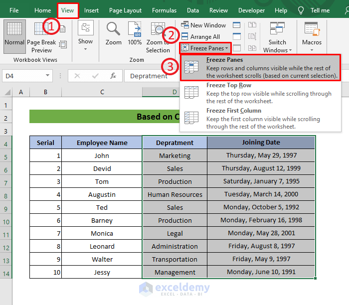
- Select the cell at the intersection where you want to freeze both rows and columns. For instance, selecting cell B4 will freeze the first three rows and the first column.
- Go to “View” > “Freeze Panes” > “Freeze Panes”.
4. Using Excel Shortcuts

To speed up the freezing process, utilize these Excel keyboard shortcuts:
| Action | Windows | Mac |
|---|---|---|
| Freeze Top Row | Alt + W, F, R | ⌘ + W, F, R |
| Freeze First Column | Alt + W, F, C | ⌘ + W, F, C |
| Freeze Panes | Alt + W, F, F | ⌘ + W, F, F |

5. Unfreezing Panes

If you need to revert back to normal scrolling, follow these steps:
- Navigate to the “View” tab on the Ribbon.
- In the “Window” group, click “Freeze Panes”.
- Select “Unfreeze Panes”.
To summarize our journey through freezing rows in Excel, we've covered multiple techniques to enhance visibility and ease of use when working with extensive data. From simple one-row freezes to freezing multiple rows, combining row and column freezes, using shortcuts, and unfreezing panes, you're now equipped to handle any spreadsheet with greater control. Remember, this feature not only maintains consistency and efficiency but also significantly improves the visibility of crucial data, allowing for more precise work.
What happens if I freeze more rows than are visible on my screen?

+
Excel will freeze the rows up to the point where they are visible on the screen. Any rows beyond the screen size will not be frozen and will scroll normally.
Can I freeze rows in Excel Online?

+
Yes, Excel Online supports freezing panes in much the same way as the desktop application. Navigate to the “View” tab to access the freeze options.
Is there a limit to how many rows I can freeze?

+
While there’s no specific limit to the number of rows you can freeze, practicality would suggest keeping the number reasonable for visibility and usability purposes.