5 Simple Steps to Link Sheets 1 and 2 in Excel

In today's fast-paced business environment, efficient data management is key to staying ahead. Microsoft Excel remains a staple for data organization and analysis, with its powerful features helping users simplify complex tasks. One such feature is the ability to link sheets within a workbook, which can streamline workflows significantly. Whether you're a financial analyst or a marketing manager, knowing how to link sheets 1 and 2 in Excel can save you considerable time and reduce the risk of errors in data management. Here are 5 simple steps to effectively link sheets within Excel:
Step 1: Identify Your Data

The first step in linking sheets in Excel involves identifying the data you wish to link. Here’s how:
- Select Sheet 1: Open your Excel workbook and click on the tab for Sheet 1.
- Select Data: Highlight the cell or range of cells you want to link. For example, if your sales figures are in cells A1 through B20, select this range.
- Sheet 2 Data: Determine where in Sheet 2 you want this data to appear. Perhaps you’re organizing a summary in Sheet 2.

🔍 Note: Make sure the data you’re linking doesn’t change frequently, as this can lead to automatic updates that might catch you off guard.
Step 2: Use the Correct Formula

With your data identified, the next step is to use a formula to create a link:
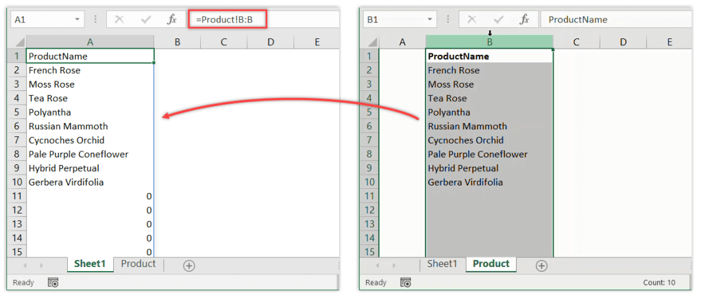
- Formula Syntax: In the cell where you want the data to appear on Sheet 2, type =Sheet1! followed by the cell reference from Sheet 1. For example, if linking cell A1 from Sheet 1 to Sheet 2, your formula would be =Sheet1!A1.
- Example: You can also link a range using the CONCATENATE function or the ampersand (&) to join multiple cells.

🔢 Note: Remember that the formula might need adjusting based on the structure of your data. Dynamic linking can be useful for large datasets.
Step 3: Copy the Link Formula

After creating the initial link, you’ll often need to link more than one cell:
- Copy: Click the cell containing the link formula.
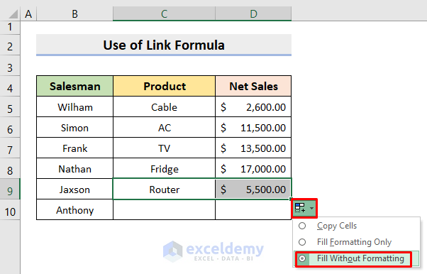
- Drag Fill Handle: Use the fill handle in the lower right corner of the cell to drag down or across to fill additional cells.

📝 Note: When copying formulas, Excel adjusts the references automatically, which is a smart function but might require manual adjustments if needed.
Step 4: Check and Test Links

Linking sheets requires a bit of quality control:
- Verify Links: Make sure all formulas link to the correct cells by clicking in each cell containing a link on Sheet 2 and checking the formula bar.
- Test Data: Enter some test data into Sheet 1 and observe the changes reflected in Sheet 2.
- Error Checking: Use Excel’s error-checking tools to find and fix any issues in your formulas.

Step 5: Finalize Your Spreadsheet

With your links successfully established, it’s time to:
- Format: Ensure all formatting is consistent across both sheets, using conditional formatting if necessary.
- Protect: You might want to protect the linked cells or entire sheets to prevent accidental changes.
- Save: Save your workbook. Keep in mind that linked sheets depend on each other, so make sure to save both.

Linking sheets in Excel is not just about saving time; it's about enhancing data integrity, reducing manual errors, and improving the overall efficiency of data handling in your projects. By following these 5 simple steps, you can create a streamlined, interconnected workbook that makes managing your data a breeze. Remember, Excel offers numerous ways to manage data, and linking sheets is just one powerful technique in your toolkit.
Can I link sheets in Excel if they’re in different workbooks?

+
Yes, you can link sheets from different workbooks using external references. Just ensure the workbooks are open when you create the links.
What happens if I delete the source sheet?

+
If you delete the source sheet, all links to it will break, resulting in #REF! errors in your linked cells on Sheet 2.
How can I update all linked data at once?

+
Use Excel’s Refresh All option under the Data tab to update all linked data simultaneously.