Linking Sheets in Excel: A Simple Guide

What is Linking in Excel?

Linking in Microsoft Excel involves creating connections between different sheets or workbooks so that when data is updated in one location, the changes automatically reflect in all linked locations. This can save a lot of time, reduce errors, and maintain data consistency. Here’s how you can do it:
Steps to Link Sheets in the Same Workbook

Select the Destination Cell: Click on the cell where you want the linked data to appear.
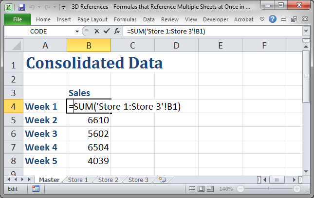
Use the Link Formula: Enter the = sign to start a formula, then switch to the source sheet. Click the cell with the data you want to link. For example, if you’re linking cell A1 from Sheet2 to Sheet1’s cell B1, you would type:
=Sheet2!A1Press Enter: Once you’ve created the link by typing the formula, hit Enter. Your destination cell will now show the value from the source cell.
🔗 Note: Remember to use absolute cell references (like $A$1) if you want to ensure the link stays fixed, even if you copy the formula.
Linking Sheets Across Different Workbooks

Linking between workbooks is similar, but you need to pay attention to file names:
Open Both Workbooks: Have the source and destination workbook open.
Select the Destination Cell: Click where you want the linked data to appear.
Type the Link Formula: Start with the equals sign (=), then type the name of the source workbook in square brackets, followed by the sheet name, and the cell reference. For example:
=[Book1.xlsx]Sheet2!A1Press Enter: Hit Enter to create the link.
🔗 Note: If you move the linked workbook, Excel will try to find the file at its new location, but links may break if it can't.
Managing Linked Sheets

To manage or troubleshoot linked sheets:
- Editing Links: Go to Data > Edit Links to manage external links. From here, you can update links, break links, or change the source.
- Refreshing Data: Right-click a linked cell and choose Refresh or press F5 to update the data manually.
- Automatic Update: Ensure the workbook is set to update automatically when opened. You can adjust this under Excel Options > Advanced under “General”.
Advanced Linking Techniques

Excel offers several advanced methods to link sheets:
Named Ranges: Instead of linking directly to cells, use named ranges. This makes formulas easier to read and maintain. To create a named range, select the cells, go to Formulas > Define Name, and name your range.
Using VLOOKUP or INDEX/MATCH: These functions can pull data dynamically from other sheets based on specific criteria, which can be useful for creating dashboards or reports.
Power Query: For advanced users, Power Query (Get & Transform in Excel) allows for more complex data connections, merging, and transformation.
To wrap up, mastering the art of linking sheets in Excel can significantly enhance productivity and data accuracy. Whether you're managing sales figures, consolidating reports, or just keeping your data organized, linking cells and workbooks helps keep everything in sync. By following the steps outlined, you'll be able to create dynamic and efficient spreadsheets that update seamlessly as your data changes.
What happens if I change the name of a linked sheet?

+
If you rename a linked sheet, Excel will automatically update the links unless the workbook is closed when you make the change. In that case, you’ll need to update the links manually when the workbook is next opened.
Can I link multiple cells at once?

+
Yes, you can link multiple cells by selecting them and dragging the fill handle (the small square in the bottom right corner of the selection) to apply the link formula to adjacent cells.
How do I find all links in my workbook?

+
To find all links, go to Data > Edit Links. This will list all external links. For internal links, you might need to manually review formulas or use the Find function to search for ‘!’ character, which usually indicates a sheet reference.