5 Simple Ways to Link Sheets in Excel 2013

Linking sheets in Excel 2013 is an essential skill for anyone who deals with complex data sets or needs to streamline their workflow. By linking sheets, you can reduce repetitive data entry, ensure consistency across documents, and make your spreadsheets more dynamic. Here are five simple ways to link sheets in Excel 2013 that will boost your productivity.
1. Using Cell References

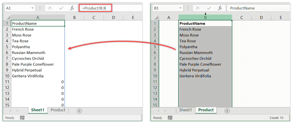
The most basic method to link data between sheets in Excel 2013 is through cell references.
- Start by selecting the cell in the destination sheet where you want the linked data to appear.
- Type ‘=’ followed by the reference to the cell from another sheet. For example, to link to cell A1 in Sheet2, you would type ‘=Sheet2!A1’.
- Press Enter, and the value of the referenced cell will appear in your current cell.
💡 Note: Remember to update cell references if you move or insert rows or columns in the source sheet, as this might break the links.
2. Named Ranges

Named ranges provide a more manageable way to link data when you have multiple references.
- Define a named range by selecting the cells you want to link and then going to ‘Formulas’ > ‘Define Name’.
- Name your range, e.g., ‘SalesData’.
- Use this name in your formula on another sheet like ‘=SalesData’ to link to the named range.
💡 Note: Using named ranges not only makes your formulas easier to read but also helps prevent errors when linking.
3. Hyperlinks

If you need to link to a specific cell, row, or section in another sheet for easy navigation, you can use hyperlinks.
- Select the cell where you want to place the hyperlink.
- Go to ‘Insert’ > ‘Hyperlink’ or press ‘Ctrl + K’.
- Under “Link to”, choose ‘Place in This Document’ and select the destination sheet and cell.
- Click ‘OK’.
💡 Note: Hyperlinks provide a visual cue for users, making navigation between sheets more intuitive.
4. 3D Formulas

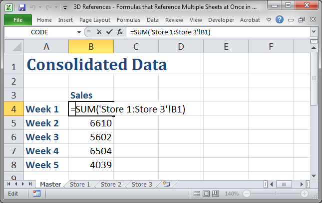
3D formulas are useful when you need to perform calculations across multiple sheets.
- Select the cell where you want the result to appear.
- Enter a formula that references multiple sheets, e.g., ‘=SUM(Sheet1:Sheet3!A1)’ to sum cell A1 from Sheet1 through Sheet3.
- Press Enter to execute the formula.
💡 Note: 3D formulas are particularly useful for summarizing data across sheets but can become complex in large workbooks.
5. Data Consolidation

For situations where you need to summarize or aggregate data from different sheets, use data consolidation.
- Go to ‘Data’ > ‘Consolidate’.
- Choose the function you want to apply (Sum, Average, Count, etc.).
- Specify the range of sheets or cells to consolidate, ensuring you select ‘Link to source data’ for dynamic updates.
- Click ‘OK’ to create a summary table that dynamically updates with source changes.
💡 Note: Data consolidation can be complex to set up, but it offers powerful summary capabilities and can be a game-changer for large datasets.
Linking sheets in Excel 2013 isn't just about saving time; it's about enhancing the integrity and flexibility of your data analysis. From simple cell references to sophisticated data consolidation, these methods provide various levels of linking that suit different needs. By mastering these techniques, you ensure that your spreadsheets are not only more efficient but also more reliable. Whether you're a financial analyst, a project manager, or anyone in between, these linking methods can significantly improve your workflow in Excel.
How do I update links when I change data in the source sheet?

+
Changes in the source sheet will automatically update linked data in all connected sheets. Ensure that the links are not broken by moving or deleting cells that contain linked data.
Can I link to external Excel workbooks?

+
Yes, you can link to external workbooks by using a similar method to internal linking, just include the workbook’s filename in the formula, like ‘=[ExternalWorkbook.xlsx]Sheet1!A1’.
What happens if I rename a sheet that is referenced in formulas?

+
If you rename a sheet, all formulas linking to that sheet will break. You’ll need to manually update the sheet names in the formulas or use Find & Replace to update multiple links at once.


