5 Easy Ways to Hyperlink Excel Cells to Another Sheet

Linking cells across different sheets in Microsoft Excel can transform your data management and analysis processes. Whether you're tracking financial data, organizing event planning details, or compiling a database, knowing how to hyperlink Excel cells to another sheet is essential for enhancing your workflow efficiency. Here are five straightforward methods to achieve this:
1. Using the HYPERLINK Function

The HYPERLINK function in Excel allows you to create a clickable link that directs to another location within your workbook.
- Select the cell where you want to insert the hyperlink.
- Type the formula:
=HYPERLINK(“#‘SheetName’!A1”, “Link Text”). - Replace ‘SheetName’ with the name of the sheet you want to link to, and ‘A1’ with the cell reference.
📌 Note: Make sure the sheet name and cell reference are correct to avoid broken links.
2. Inserting Hyperlinks Manually

If you prefer not to use formulas, you can manually insert hyperlinks:
- Right-click on the cell where you want to insert the link.
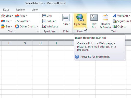
- Select ‘Hyperlink’ or press Ctrl+K.
- Choose “Place in This Document” and navigate to your desired cell on another sheet.
3. Creating Hyperlinks with VBA

For those comfortable with macros, VBA (Visual Basic for Applications) provides a dynamic way to manage hyperlinks:
Sub AddHyperlink()
    ActiveCell.Hyperlinks.Add Anchor:=Selection, Address:=“”, SubAddress:=“‘SheetName’!A1”, TextToDisplay:=“Link Text”
End Sub
Assign this macro to a button or run it from the VBA editor. Replace ‘SheetName’ and ‘A1’ with your specific references.
💡 Note: You need to enable macros to use VBA in your Excel workbook.
4. Using Name Manager for More Complex Links

The Name Manager in Excel can help create references that can be used as hyperlinks:
- Go to the Formulas tab and click ‘Name Manager’.
- Create a name that refers to the cell or range you want to link to.
- Use this named reference in a hyperlink formula like
=HYPERLINK(“#NamedRange”, “Link Text”).
This method is particularly useful for linking to dynamic ranges or areas that might change over time.
5. Conditional Hyperlinks

To create hyperlinks based on conditions:
- Use an IF statement combined with HYPERLINK:
=IF(A1=“Condition”, HYPERLINK(“#‘SheetName’!A1”, “Text”), “No Link”)
The ability to hyperlink cells in Excel to different sheets is a game-changer for data organization and navigation. By mastering these methods, from simple HYPERLINK functions to more advanced VBA scripting, you can significantly improve your efficiency in handling large and complex workbooks. The techniques range from static to dynamic hyperlinks, catering to various levels of Excel proficiency. Remember to ensure that your sheet names and cell references are accurate to avoid errors in your linking process.
What is the benefit of using the HYPERLINK function?

+
The HYPERLINK function in Excel allows users to create interactive links to other parts of the workbook or external files, facilitating quick navigation and data interaction.
Can you make a hyperlink appear only if a certain condition is met?

+
Yes, by combining the IF statement with HYPERLINK, you can create conditional hyperlinks that appear based on specific criteria.
How do you update a hyperlink if the sheet name changes?

+
You need to manually update the sheet name in the hyperlink formula or use named ranges that automatically adjust if the sheet is renamed.
What should I do if my VBA hyperlink macro doesn’t work?

+
Ensure that macros are enabled in your Excel settings, and check for any typos in the VBA code. Also, verify that the macro is correctly assigned to a button or hotkey.