Master Excel: Highlight Cells Like a Pro

How to Master Excel: Highlight Cells Like a Pro

Excel is an incredibly powerful tool for organizing, analyzing, and presenting data. One of the key features that makes Excel versatile for both beginners and experts alike is the ability to highlight cells in various ways. Whether you're using conditional formatting to highlight anomalies, applying dynamic colors to enhance data visualization, or just setting up custom styles to distinguish between different types of data, Excel's cell highlighting features can significantly boost your productivity and the clarity of your spreadsheets. Here’s how you can start highlighting cells like a pro:

Understanding the Basics of Cell Highlighting

Before diving into advanced techniques, let's go over the basics:

• Manual Highlighting: Right-click on a cell or select a range, then choose Format Cells to manually change fill colors.
• Quick Access Toolbar: Add the Format Painter to your toolbar for quick color copy-paste operations.
• Predefined Styles: Excel comes with a variety of predefined cell styles that can quickly highlight cells based on common criteria.

Conditional Formatting

Conditional Formatting in Excel allows you to highlight cells that meet certain criteria, making it easier to analyze data. Here’s how you can use it:

Using Predefined Rules

1. Select the range of cells you want to format.
2. Go to Home > Conditional Formatting > Highlight Cells Rules.
3. Choose the rule you need (e.g., Greater Than, Less Than, Between, etc.).
4. Set your criteria and choose a formatting style.

Example:

💡 Note: To apply conditional formatting, you must select the cells first before navigating to the Conditional Formatting menu.

Custom Formatting

For more personalized data highlighting, custom formatting is the way to go:

• Using Formulas: Enter a formula to define when cells should be formatted.
• Data Bars, Color Scales, Icon Sets: These visual elements can add an extra layer of readability to your data.

Advanced Techniques

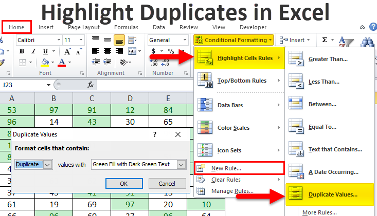
Highlighting Duplicate Values

To find and highlight duplicates:

1. Select the range where you want to find duplicates.
2. Navigate to Home > Conditional Formatting > Highlight Cells Rules > Duplicate Values.
3. Choose the color to highlight duplicates.

Using VBA for Custom Highlighting

For those comfortable with VBA, scripting can automate highlighting in complex ways:

Sub HighlightWithCondition()
    'This script highlights cells based on custom conditions
    Dim rng As Range
    Set rng = Selection
    For Each cell In rng
        If cell.Value > 100 Then
            cell.Interior.Color = RGB(255, 255, 0) 'Yellow
        ElseIf cell.Value < 0 Then
            cell.Interior.Color = RGB(255, 0, 0)   'Red
        End If
    Next cell
End Sub

Tips for Effective Highlighting

• Be Consistent: Use a color scheme that consistently represents similar data types.
• Less is More: Overuse of colors can clutter your spreadsheet. Use highlighting sparingly for the most important information.
• Accessibility: Remember that not everyone perceives colors in the same way. Consider using patterns or icons alongside colors.

🌟 Note: When using conditional formatting, always check for overlapping conditions to ensure expected results.

In mastering Excel’s cell highlighting, you’ve unlocked a valuable tool for data analysis and presentation. By applying these techniques, you can:

• Quickly identify trends or anomalies in your data.
• Make your spreadsheets more visually appealing and easier to interpret.
• Automate data processing with custom VBA scripts for recurring tasks.

There’s a wealth of knowledge waiting to be explored with Excel. From simple color changes to complex conditional formatting, the ability to highlight cells effectively can transform how you work with data.

Wrapping Up:

From understanding the fundamental methods of cell highlighting to leveraging conditional formatting and VBA scripting, this guide has covered how you can use Excel to present and analyze data in visually appealing ways. Remember to practice these skills on real data sets, as real-world application will solidify your understanding and make these techniques second nature.

Can I highlight cells based on multiple conditions?

+

Yes, you can! Conditional Formatting in Excel supports applying multiple conditions to the same range. Each condition will format the cells if they meet its criteria, but you can use priority (by ordering rules) to ensure one condition doesn’t override another unless necessary.

What if I want to highlight a cell if it matches a value from another cell or range?

+

You can use the Use a formula to determine which cells to format option under Conditional Formatting. Enter a formula like =A1=B1 or =A1=E1 (if B1 or E1 is the reference cell) to achieve this.

How can I remove conditional formatting from my cells?

+

Select the cells with conditional formatting, go to Home > Conditional Formatting > Clear Rules > Clear Rules from Selected Cells.