Highlight Excel Cells: Easy Techniques for Beginners

Learning how to highlight cells in Excel is essential for anyone starting to explore the power of spreadsheets. Not only does it improve the visual appeal of your data, but it also aids in quickly identifying important information. In this post, we'll go through some of the most straightforward techniques beginners can use to enhance their Excel workbooks with color.
Manual Cell Highlighting

The simplest way to highlight cells in Excel is through manual selection. Here's how you can do it:
- Select the cells you want to highlight by clicking and dragging your mouse over them.
- Go to the Home tab on the Excel Ribbon.
- In the Font group, click the Fill Color icon (a paint bucket).
- Choose your preferred color from the palette.
⚠️ Note: Be careful not to choose a color that might interfere with cell text visibility.
Using the Format Cells Dialog Box

If you need more control over the colors or want to apply different patterns, the Format Cells dialog box is the way to go:
- Select the cells you wish to format.
- Right-click and choose Format Cells, or press Ctrl + 1.
- Go to the Fill tab.
- Select a color or a pattern, and adjust the pattern color if applicable.
- Click OK to apply.
Conditional Formatting for Dynamic Highlighting

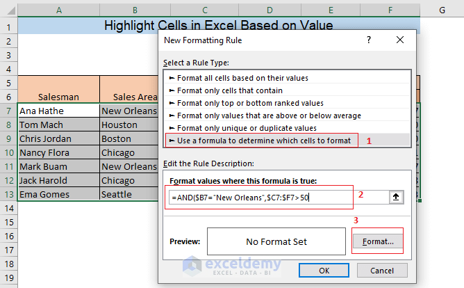
Conditional formatting is a powerful tool that highlights cells based on certain criteria, making data analysis effortless:
- Select your data range.
- Go to Home > Conditional Formatting.
- Choose from various options like Highlight Cells Rules, Top/Bottom Rules, or Color Scales.
- Set the rules, and Excel will apply color based on the conditions you've set.
Highlighting Duplicates

To make duplicates stand out, you can use conditional formatting as follows:
- Select the range where you want to find duplicates.
- Go to Home > Conditional Formatting > Highlight Cells Rules > Duplicate Values.
- Choose the color you want to use to highlight duplicates.
Color Schemes for Easy Navigation

Using color schemes can help in distinguishing different categories of data:
- Select your data set.
- Go to Home > Format as Table.
- Choose a color scheme that suits your needs. Excel will color the headers and apply alternating row colors for better readability.
📚 Note: Tables in Excel not only help with navigation but also make it easier to manage and analyze data through built-in features like filters and sorting.
Conclusion

Mastering the art of cell highlighting in Excel can significantly improve how you present and analyze data. From simple manual selections to dynamic conditional formatting, Excel offers a plethora of options to ensure your work stands out. Keep in mind that while highlighting can make your spreadsheet visually appealing, it should also serve a functional purpose, enhancing the readability and analysis of your data.
How do I remove highlight color from cells?

+
Select the highlighted cells, go to the Home tab, and click on the Fill Color icon. Choose “No Fill” to remove the color.
Can I highlight cells based on their text content?

+
Yes, using conditional formatting, you can highlight cells containing specific text, numbers, or even using custom formulas to determine what to highlight.
What if I want to highlight an entire row or column?

+
To highlight an entire row or column, select it by clicking on the row number or column letter. Then use the Fill Color tool or apply conditional formatting rules as needed.