Freeze Top 3 Rows in Excel: A Quick Guide

When dealing with large datasets in Microsoft Excel, it can be challenging to keep track of your headers and key rows as you scroll through your data. Fortunately, Excel provides a Freeze Panes feature which allows you to freeze the top rows or columns of your spreadsheet, ensuring that your headers remain visible no matter how far down or across you scroll. This guide will walk you through how to freeze the top three rows in Excel, which can significantly improve your data navigation and analysis experience.
Why Freeze Rows?

- Visibility: Keeps crucial information like headers or summary rows always in view, regardless of how much you scroll.
- Orientation: Ensures you don't lose context when dealing with extensive datasets.
- Efficiency: Reduces the time you spend scrolling up and down to remind yourself of column headers or important data.
How to Freeze Top 3 Rows in Excel

Freezing the top three rows in Excel is straightforward:
Step 1: Open Your Excel Workbook

- Open Microsoft Excel and your workbook containing the data you wish to work with.
Step 2: Navigate to the View Tab

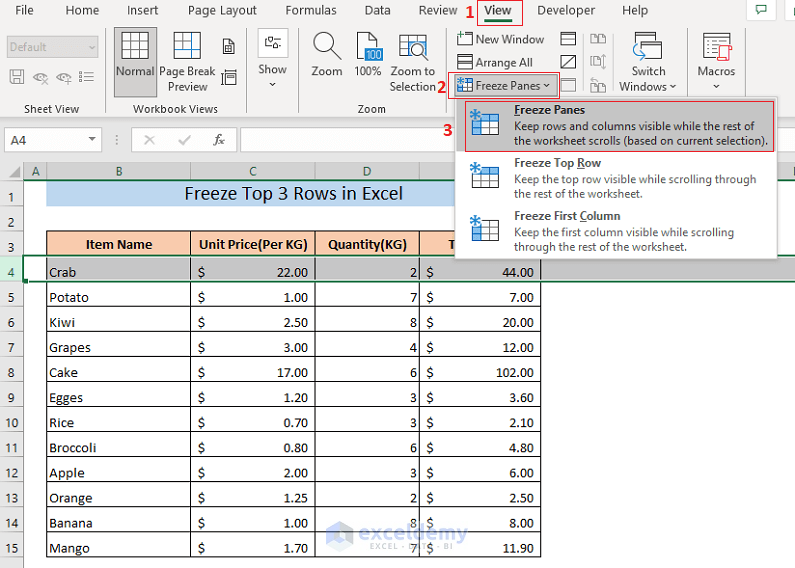
- Go to the View tab on the Excel ribbon, which contains various options for how you view your workbook.
Step 3: Freeze the Top Rows

- In the Window group, find the Freeze Panes option. Here, you have three choices:
- Freeze Panes: Freezes panes based on your current cell selection.
- Freeze Top Row: Freezes the very top row.
- Freeze First Column: Freezes the first column on the left.
- Click on Freeze Panes, and then select Freeze Panes from the dropdown menu. This will freeze the top three rows if your cursor is in the cell below the third row (e.g., cell A4).
Step 4: Verify the Rows are Frozen

- Scroll down through your data to check that the top three rows are indeed frozen at the top of your window. You should see lines indicating the freeze boundary.
🚧 Note: Excel freezes panes based on the active cell's position. If you select a cell in the fourth row, Excel will freeze the three rows above that cell.
Unfreeze Panes

If you decide to unfreeze the panes:
- Go back to the View tab and select Unfreeze Panes from the Freeze Panes dropdown.
Advanced Tips for Freezing Panes

- Freezing Both Rows and Columns: Position your cursor in the cell below the rows you want to freeze and to the right of the columns. For instance, cell B4 would freeze the first three rows and column A.
- Dynamic Freeze: If your dataset expands or contracts, you can dynamically adjust which rows are frozen by changing the active cell’s position and re-applying the freeze function.
- Keyboard Shortcut: For a quicker freeze, use the keyboard shortcut: Windows: Alt + W + F + F or Mac: Command + Option + W, F.
In conclusion, mastering the art of freezing panes in Excel can transform the way you work with data. Not only does it make navigation simpler, but it also helps in maintaining focus on key information. Whether you’re a data analyst, a project manager, or just someone dealing with large spreadsheets, freezing panes ensures that your most important data is always in sight, making your workflow smoother and more efficient.
Can I freeze panes in Google Sheets?

+
Yes, you can freeze panes in Google Sheets using the ‘View’ menu or by dragging the gray bar above row 1 or left of column A.
What if I need to freeze more than three rows?

+
You can freeze as many rows as you like by selecting the row below the last row you wish to freeze and then using the ‘Freeze Panes’ option.
Does freezing panes affect the printing of my spreadsheet?

+
No, freezing panes is only for the on-screen display. Printing settings must be adjusted separately.