Freeze Sheets in Excel 2010: Step-by-Step Guide

Unlocking the Potential of Excel 2010: A Comprehensive Guide to Freezing Sheets

Excel 2010 offers an array of features that make managing and analyzing data an effortless task. Among these, the ability to freeze rows and columns can significantly enhance your data handling. This guide will walk you through the steps to freeze panes in Excel 2010, ensuring you can navigate through your spreadsheets with ease, maintaining your focus on essential data points.
Understanding the Need for Freezing Sheets

Freezing sheets is all about keeping a certain number of rows or columns always visible on the screen as you scroll. This is particularly useful when dealing with extensive datasets where headers or key columns need to remain in view to provide context for the data being analyzed. By freezing these elements, you make navigation smoother and data interpretation more intuitive.
Step-by-Step Guide to Freeze Sheets

Let's dive into the step-by-step process of freezing sheets in Excel 2010:
Step 1: Open Your Excel Document

Start by launching Microsoft Excel 2010 and opening the workbook where you want to apply the freeze function.
Step 2: Select Your Freeze Point

Determine the row or column after which you want to freeze the data. For example, if you want the first row to remain fixed at the top while scrolling, you'd select the cell directly below it.
🔍 Note: You can freeze both rows and columns simultaneously by selecting a cell that is directly below the row and to the right of the column you want to freeze.
Step 3: Access the Freeze Panes Option

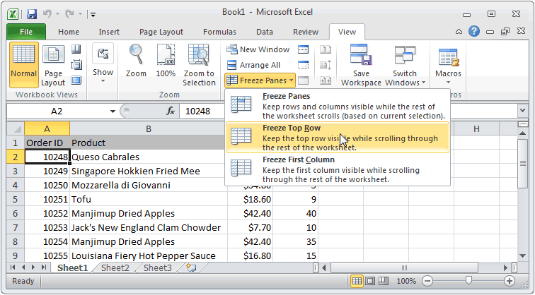
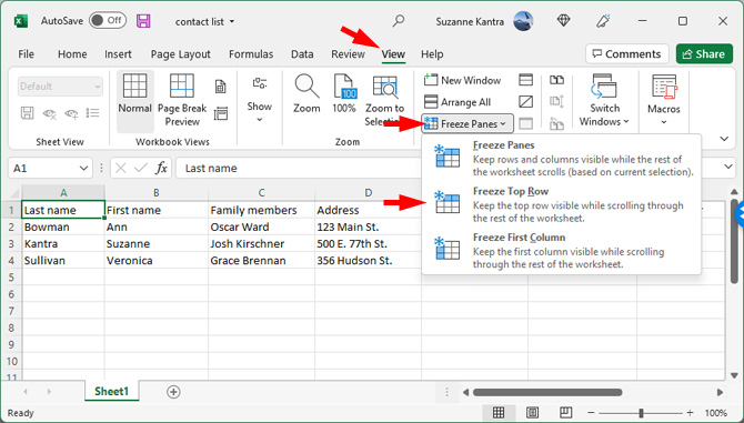
- Navigate to the View tab on the Ribbon.
- Click on the Freeze Panes button in the Window group.
- From the dropdown menu, choose one of the following:
- Freeze Panes to freeze panes based on your selected cell.
- Freeze Top Row to freeze the first row.
- Freeze First Column to freeze the leftmost column.
Step 4: Verify the Freezing

After selecting the freeze option, you'll notice horizontal or vertical lines appearing on the sheet, indicating which parts are fixed in place. Scroll to see if the selected rows or columns remain in view.
Step 5: Unfreeze Panes if Necessary

To unfreeze panes, revisit the View tab, click on Freeze Panes, and select Unfreeze Panes.
Advanced Tips for Excel Panes

Freezing panes in Excel 2010 opens up numerous possibilities for data management. Here are some tips:
Freezing Multiple Rows or Columns

- To freeze multiple rows or columns, select the row or column below or to the right of where you want the freeze to start.
- Using the Freeze Panes option, Excel will freeze all rows above and all columns to the left of the selected cell.
Using Tables

| Option | Description |
|---|---|
| Freeze Top Row | Fixes the top row in view when scrolling vertically. |
| Freeze First Column | Keeps the first column in view when scrolling horizontally. |
| Freeze Panes | Freezes all rows and columns above and to the left of the selected cell. |

Wrapping Up the Guide

Mastering the art of freezing sheets in Excel 2010 can dramatically improve your data analysis workflow. Whether you're dealing with financial models, inventory lists, or any other data-intensive task, keeping your headers or important reference columns in view will streamline your work, reducing the time spent on scrolling back and forth.
Can I freeze both rows and columns at the same time in Excel 2010?

+
Yes, you can freeze both rows and columns simultaneously by selecting the cell that lies directly below the last row you want to freeze and directly to the right of the last column you want to freeze.
What is the difference between Freeze Panes and Freeze Top Row in Excel?

+
Freeze Panes allows you to freeze rows and columns up to the cell you’ve selected, whereas Freeze Top Row will only lock the top row in place when scrolling.
How do I know which rows or columns are frozen?

+
When you apply the freeze, Excel will display a gray line to indicate where the frozen pane ends. This line moves with you as you scroll through your spreadsheet.