How to Freeze Rows in Excel: Easy Guide

When working with large sets of data in Microsoft Excel, it often becomes crucial to maintain visibility of headers or key rows as you scroll through your spreadsheet. Freezing rows in Excel can enhance your productivity by keeping important information in view, no matter how far down you scroll. Here's an easy guide to get you started:
Why Freeze Rows?

Freezing rows in Excel is particularly useful for:
- Keeping Headers Visible: For extensive datasets where you need to constantly see column headers or specific row labels.
- Comparing Data: When comparing data spread over multiple pages or sections of a worksheet.
- Presentations: To ensure that key information remains on-screen during presentations or meetings.

How to Freeze Rows in Excel

Freezing rows in Excel can be achieved through several steps:
Using the "Freeze Panes" Feature

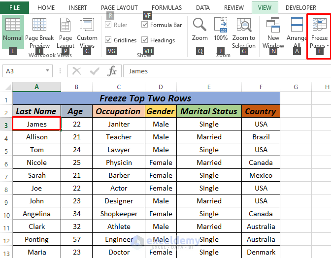
- Select the Row Below: Click on the row number of the row directly below the one you want to freeze. If you want to freeze the first row, click on the row number 2.
- Navigate to the View Tab: On the Excel ribbon, select the "View" tab.
- Choose Freeze Panes: Within the "View" tab, find the "Freeze Panes" button in the "Window" group. Click it, then select either:
- "Freeze Panes" to freeze the selected row above
- "Freeze Top Row" if you want to specifically freeze the top row
- Verify the Freeze: Scroll down to check that the row remains at the top of your view.
Using Keyboard Shortcuts

While there isn't a specific shortcut for freezing panes directly, you can speed up the process:
- Ctrl + G: Use this to quickly navigate to a specific cell or row.
- Ctrl + End: This will take you to the last cell of your data.
- Follow the Steps: Once there, follow the steps mentioned above.
Freeze Multiple Rows

To freeze multiple rows, you select the row below the last row you want to freeze:
- Select Row: Click on the row number below the last row you wish to freeze.
- Freeze: From the "View" tab, select "Freeze Panes" then "Freeze Panes" again.
Notes on Freezing Rows

⚠️ Note: Remember that freezing rows affects the scrolling behavior across the entire worksheet.
Unfreezing Rows

If you need to revert to normal scrolling:
- Navigate to View: Go to the "View" tab.
- Freeze Panes: In the "Window" group, select "Unfreeze Panes".
Advanced Techniques

Sometimes, you might need to freeze both rows and columns together:
- Select Cell: Click on the cell that is immediately to the right of the column you want to freeze and below the row you want to freeze.
- Freeze Panes: From the "View" tab, choose "Freeze Panes" to lock both the rows above and the columns to the left of the selected cell.
This ensures that when you scroll, headers and the first column (if needed) remain visible, enhancing your ability to navigate through complex spreadsheets.
✅ Note: Freezing panes is not available in the web version of Excel, but the desktop version of Excel provides these options.
By following these steps, freezing rows in Excel becomes an intuitive task that significantly improves your ability to manage and analyze data effectively. Whether you're dealing with financial records, project management, or any large dataset, keeping key information in view can make your workflow much smoother.
How many rows can I freeze in Excel?

+
You can freeze as many rows as you need, up to the total number of rows in your Excel worksheet, which is 1,048,576 in newer versions. However, freezing too many rows might reduce the effective workspace on your screen.
What happens to frozen rows when I insert new rows?

+
If you insert new rows above the frozen section, Excel will adjust the freeze, moving it to encompass the new rows if necessary. If you want to ensure certain rows are always frozen, you’ll need to manually update the freeze after adding or removing rows.
Can I freeze both rows and columns?

+
Yes, you can freeze rows and columns together by selecting the cell that is below the last row you want to freeze and to the right of the last column you want to freeze before choosing “Freeze Panes.”