5 Ways to Freeze Half of an Excel Sheet

When working with Excel, there might be occasions when you need to focus on a specific section of your spreadsheet while keeping other parts easily accessible. By freezing half of an Excel sheet, you can lock rows or columns in place to ensure that the headers or key information remains visible as you scroll through larger datasets. Here are five methods to achieve this:
Method 1: Freezing Panes

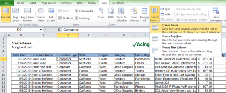
Freezing panes in Excel allows you to lock rows and columns:
- Select the cell below the row(s) and to the right of the column(s) you want to freeze.
- Go to the View tab.
- Click on Freeze Panes and choose from the options:
- Freeze Panes
- Freeze Top Row
- Freeze First Column
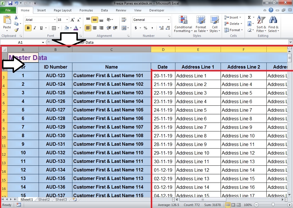
Your Excel sheet will now display lines to indicate where the panes are frozen.
Method 2: Split Window

The split window feature in Excel lets you view different parts of your worksheet simultaneously:
- Move your cursor to the scroll bars until it changes to a double-headed arrow.
- Click and drag to create a split. You can split the window both horizontally and vertically.
- Use the scroll bars to navigate through each pane independently.
📘 Note: The split window technique does not lock panes; it allows for independent scrolling.
Method 3: Locking Cells

If you need to prevent others from editing specific parts of your worksheet, you can:
- Select the cells or range you wish to lock.
- Go to Home tab, click on Format, then Protect Sheet.
- Check Lock cells and set up passwords if needed.
This method prevents changes but does not freeze the visual aspect of the sheet.
Method 4: View Side by Side

While this method isn't for freezing, it provides a similar effect:
- Open two instances of the same Excel file.
- Go to View, click New Window, and then choose View Side by Side.
- Each window can be independently scrolled to display different sections of the sheet.
Method 5: VBA Macro for Partial Freeze

For advanced users, VBA offers a way to partially freeze a sheet:
- Open the VBA editor by pressing Alt + F11.
- Insert a new module and paste the following code:
Sub PartialFreeze() ActiveWindow.FreezePanes = False Rows("1:10").Select ActiveWindow.FreezePanes = True End Sub - Run this macro to freeze the first 10 rows.
This code can be adjusted to freeze any number of rows or columns as needed.
In summary, Excel provides various methods to manage your worksheet view for improved efficiency:
- Freezing panes to lock rows and columns.
- Using split windows for simultaneous viewing.
- Locking cells to prevent edits.
- Viewing sheets side by side.
- Utilizing VBA for custom freezing effects.
Each approach serves different needs, from simple navigation to more complex workbook management. Choose the method that best suits your task, and keep your data well-organized and easily accessible.
What is the difference between freezing panes and locking cells in Excel?

+
Freezing panes in Excel keeps specific rows or columns visible while scrolling, whereas locking cells secures them against edits by setting a password. This prevents modifications but doesn’t freeze the view.
Can I freeze more than one row or column in Excel?

+
Yes, you can freeze multiple rows or columns by selecting the cell below and to the right of the area you want frozen, then using the Freeze Panes command.
Is there a way to partially freeze a sheet without using VBA?

+
No, for partial freezing beyond simple rows or columns, VBA is the only way to customize the freeze functionality.
Can I still edit data in a frozen area?

+
Yes, freezing panes only affects visibility, not the ability to edit. However, locked cells require passwords to edit.
How do I revert the freeze or split in Excel?

+
To unfreeze panes, go to the View tab and select Unfreeze Panes. To remove a split, simply drag the split bar back to its original position or double-click it.