3 Simple Ways to Freeze Cells in Excel Instantly

In today's digital workplace, mastering Excel's functionalities is akin to wielding a superpower. Among the myriad of tools Excel offers, the ability to freeze specific rows or columns is invaluable, especially when dealing with large datasets. Freezing cells in Excel helps you keep important information in view, making navigation through extensive spreadsheets a breeze. Here are three simple, yet powerful ways to freeze cells in Excel:
Method 1: The Simple Freeze Panes

The Freeze Panes feature in Excel is one of the most straightforward methods to keep your headings or key columns visible:
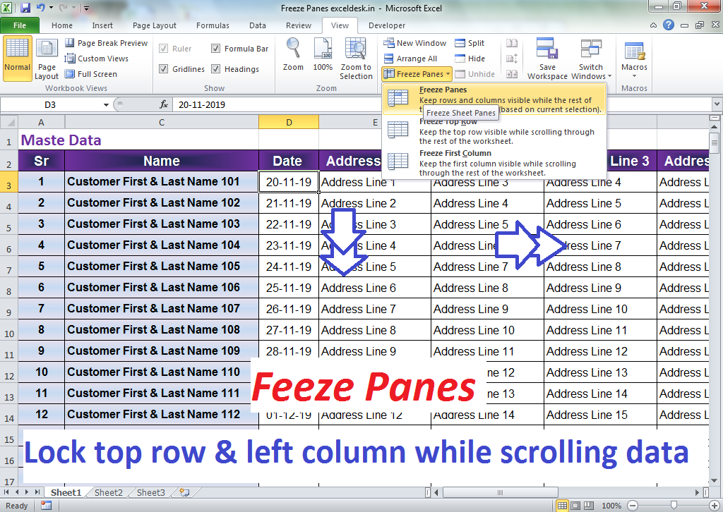
- Freeze Top Row: This option locks the top row of your worksheet in place, allowing the rest of the data to scroll beneath it.
- Freeze First Column: This locks the leftmost column, which is beneficial for spreadsheets with a fixed vertical reference.
- Freeze Panes: For more flexibility, select a cell, and Excel will freeze all rows above and columns to the left of this selection.
To apply this feature:
- Select the cell below and to the right of the rows and columns you wish to freeze.
- Navigate to the View tab in the Ribbon.
- Click on Freeze Panes, then choose your desired freeze option from the dropdown menu.
✏️ Note: Ensure you select the correct cell before using 'Freeze Panes'; otherwise, you might freeze an unintended part of your worksheet.
Method 2: Freezing Multiple Rows or Columns

Sometimes, you might need to keep more than just one row or column visible while scrolling through your data:
- Select the row below where you want the freeze to begin or the column to the right.
- Follow the same steps as with the Simple Freeze Panes, but instead of choosing the single row or column options, select Freeze Panes again to freeze multiple rows or columns.
Here's how to do it:
- Click on the row number (on the left) or the column letter (at the top) to select the entire row or column where you want to initiate the freeze.
- Go to the View tab and click Freeze Panes.
🧐 Note: Remember, freezing multiple rows or columns might obscure other data, so use this method judiciously based on your dataset size and complexity.
Method 3: Split Window View

While not traditional freezing, Split offers a dynamic view alternative:
- Split Horizontally: This feature divides the window into two scrollable parts horizontally.
- Split Vertically: Splits the window vertically, allowing for separate scrolling.
Here's how you can achieve this:
- Place your cursor over the split bar between column letters or row numbers until the cursor changes to a double-headed arrow.
- Double-click or drag the split bar to set the split at a desired point.
- Each pane can now scroll independently.
💡 Note: Splitting is great for comparing distant parts of your worksheet without needing to freeze anything permanently.
Summing it all up, knowing how to freeze cells in Excel gives you control over how you view and analyze your data. Whether you need to keep headings in sight or compare different sections of your data simultaneously, these techniques provide the flexibility you need. Each method serves its own purpose, making your Excel experience smooth and efficient. Remember, practice is key; the more you work with these features, the more intuitively you'll apply them to your worksheets.
Can I unfreeze cells in Excel?

+
Yes, you can unfreeze cells by selecting the ‘Unfreeze Panes’ option from the same ‘Freeze Panes’ dropdown menu under the View tab.
What should I do if freezing cells disrupts my spreadsheet layout?

+
Try selecting a different cell for freezing or adjust the split lines to ensure that your worksheet remains readable and organized.
Is there a limit to how many rows or columns I can freeze?

+
There isn’t a specific limit on rows or columns, but freezing too many can make navigation cumbersome. Typically, it’s best to keep it to a few rows or columns.