5 Easy Ways to Match Values Across Excel Sheets

Ever found yourself needing to compare data across multiple Excel sheets but were bogged down by the complexity of the task? Whether you're trying to reconcile financial records, validate data entries, or simply want to merge information, Excel has built-in tools and techniques to make this process seamless. This comprehensive guide will walk you through five easy-to-implement methods to match values across Excel sheets effectively. These methods are designed to not only save you time but also ensure accuracy in your data analysis tasks.

Using VLOOKUP for Quick Value Matching

One of the simplest and most effective ways to match values across different sheets in Excel is by using the VLOOKUP function. This function is ideal when you want to search for a value in one sheet and return a corresponding value from another sheet.

• Step 1: Identify the column that contains the lookup value in both sheets.
• Step 2: Use VLOOKUP with the following syntax: =VLOOKUP(lookup_value, table_array, col_index_num, [range_lookup])
• Step 3: Enter the lookup value from your source sheet into the first argument.
• Step 4: Define the table array from the sheet you want to match from.
• Step 5: Specify the column number in the table array where the matching value should be returned.
• Step 6: Set the range lookup to FALSE for an exact match.

🔎 Note: Ensure the lookup column in the source sheet has unique values for VLOOKUP to work accurately.

Employing INDEX and MATCH for Flexible Matching

While VLOOKUP is straightforward, it has limitations like its inability to look to the left. The INDEX and MATCH combination provides more flexibility.

• Step 1: Use MATCH to find the position of the lookup value within the lookup array.
• Step 2: Apply INDEX to retrieve the value from the identified position.
• Step 3: The formula structure would be: =INDEX(array, MATCH(lookup_value, lookup_array, 0))

💡 Note: INDEX and MATCH work together to overcome VLOOKUP's limitations, allowing for both vertical and horizontal lookups.

Harnessing Power Query for Advanced Matching

Power Query in Excel is a powerful tool for data transformation and consolidation. Here's how you can use it for matching values across sheets:

• Step 1: Select a cell in your source sheet.
• Step 2: Go to the Data tab, click on Get & Transform Data, then choose From Table/Range.
• Step 3: In Power Query Editor, add the second sheet by clicking Get Data and selecting the other sheet.
• Step 4: Use the Merge Queries feature to combine data based on a common field.
• Step 5: Select the join type and choose the columns to match on.
• Step 6: Click OK to merge and expand the combined data.

🛠️ Note: Power Query provides an interactive environment for data manipulation, enhancing your ability to manage complex datasets.

Leveraging Conditional Formatting for Visual Matching

Sometimes, visual cues can help identify matching or mismatching values easily:

• Step 1: Select the range in your source sheet where you want to highlight matches.
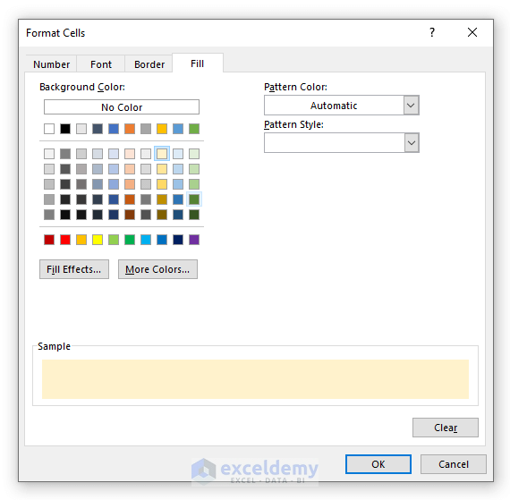
• Step 2: Go to Home > Conditional Formatting > New Rule.
• Step 3: Choose "Use a formula to determine which cells to format."
• Step 4: Input the formula using cell references from both sheets, for example: =A2=Sheet2!A2
• Step 5: Set the formatting style to highlight matches or mismatches.

👀 Note: Conditional Formatting provides an instant visual feedback, which can be very helpful for quick overviews.

Using Macros for Automated Matching

For repetitive or complex matching tasks, consider using VBA macros:

• Step 1: Press Alt+F11 to open the VBA editor.
• Step 2: Insert a new module and write a script to automate the matching process.
• Step 3: Use loops to compare cells across sheets and perform actions based on matches or mismatches.
• Step 4: Assign the macro to a button or run it directly from the VBA editor.

🧪 Note: Macros can be customized to fit any matching scenario, from simple value comparison to complex data manipulation.

Wrapping Up

Through the methods described, Excel becomes an even more powerful tool for data analysis and management. Whether you choose the straightforward VLOOKUP for simplicity, the dynamic INDEX and MATCH for flexibility, or harness the transformative capabilities of Power Query, matching values across sheets can be done efficiently and accurately. Conditional formatting provides visual aids, while macros offer automation for repetitive tasks. Mastering these techniques allows you to streamline your workflow, reduce errors, and make more informed decisions based on accurate data.

What are the limitations of VLOOKUP?

+

VLOOKUP has several limitations, including only being able to look to the right of the lookup column, its inability to handle multiple matches, and the need for an exact match unless specified otherwise.

Can I match values if there are blank cells?

+

Yes, you can use conditional formatting or VBA to handle matching values even with blank cells. Ensure to account for these in your logic.

Is Power Query available in all versions of Excel?

+

Power Query is available in Excel 2016 and later versions, including Office 365. For earlier versions, you might need to install Power Query as an add-in.

How can I learn more about VBA?

+

To learn more about VBA, you can explore online courses, Excel forums, or read books on VBA programming tailored for Excel users.