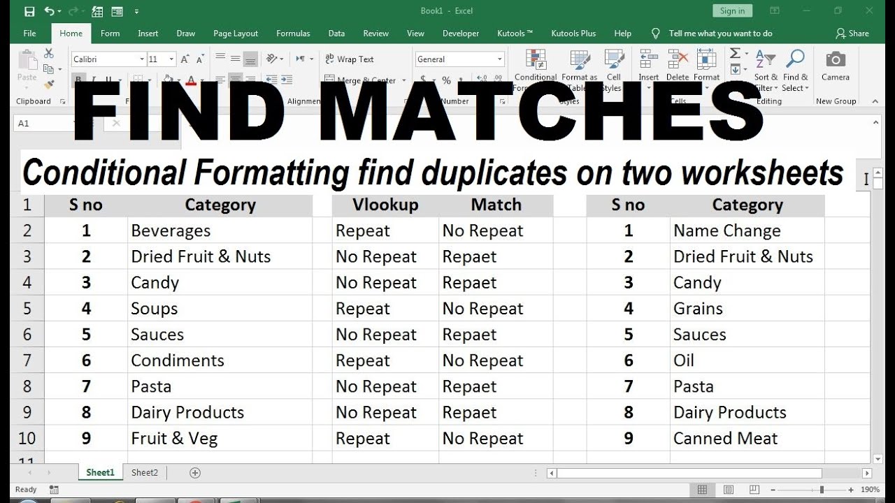
5 Easy Steps to Match Data Across Two Excel Sheets

Data matching across two Excel sheets can be a daunting task, especially when you're dealing with large datasets. However, with the right techniques, you can streamline the process to ensure accuracy and efficiency. Here are five straightforward steps to help you match data efficiently.
Step 1: Prepare Your Data


The first step in any data matching project is to ensure that your data is clean and organized:
- Review Your Data: Check for any errors or inconsistencies.
- Remove Duplicates: Use Excel’s “Remove Duplicates” feature to ensure each record is unique.
- Standardize Formats: Make sure dates, numbers, and text formats are consistent.
Step 2: Use VLOOKUP Function

The VLOOKUP function is essential for simple matching tasks. Here’s how to use it:
- Enter the formula:
=VLOOKUP(lookup_value, table_array, col_index_num, [range_lookup]) - lookup_value: This is what you want to find (e.g., an employee ID).
- table_array: The range of cells that contains the data you want to search.
- col_index_num: The column number in the table array from which to retrieve the value.
- range_lookup: Set this to FALSE for exact matches.
🚦 Note: The VLOOKUP function only searches from left to right.
Step 3: Implement INDEX and MATCH

For more flexibility, use the combination of INDEX and MATCH functions:
- MATCH: Find the position of a lookup value within a row, column, or range.
- INDEX: Return the value of a cell in a list or array, based on the numeric position.
=INDEX(return_range, MATCH(lookup_value, lookup_range, match_type))
This method allows for:
- Matching data both vertically and horizontally.
- Dynamic lookup values, enhancing flexibility.
Step 4: Leverage Power Query


Power Query offers advanced data transformation capabilities:
- Load both sheets into Power Query.
- Merge: Use the "Merge Queries" feature to join datasets based on a common key.
- Advanced Transformations: Filter, sort, or group the merged data to match your needs.
🚀 Note: Power Query can also handle large datasets with ease, making it ideal for extensive data matching tasks.
Step 5: Use Conditional Formatting for Visual Matching

If visual comparison helps you, Excel’s conditional formatting can be an ally:
- Select the range to format.
- Choose “Conditional Formatting” from the Home tab.
- Select “Highlight Cell Rules” and then “Duplicate Values” for easy visual comparison.
In conclusion, matching data between two Excel sheets is made manageable through a combination of preparation, function utilization, and advanced Excel features like Power Query. Each step builds upon the last, providing you with robust methods to ensure your data matches perfectly, saving time and reducing errors.
What if my data doesn’t match using VLOOKUP?

+
If VLOOKUP fails, ensure your lookup value is in the first column of the table array or check for any formatting issues or errors in the data. Alternatively, try using INDEX and MATCH for more flexibility.
Can I match data across multiple sheets at once?

+
Yes, with Power Query, you can merge data from multiple sheets or even different workbooks into one coherent dataset for matching.
How can I ensure data integrity when merging large datasets?

+
Always back up your data before operations. Use Power Query to perform complex transformations and merges with precision. Also, validate data post-merge to ensure no critical information was lost or misaligned.
What are the limitations of using conditional formatting for data matching?

+
Conditional formatting highlights visual discrepancies but doesn’t address or resolve underlying data issues like duplicates or missing records. It’s more a tool for visual identification rather than data correction.
Is there a method to match data without knowing the exact column order?

+
The INDEX and MATCH functions together allow you to match data without relying on a specific column order, making it versatile for handling varying structures in spreadsheets.