5 Simple Steps for VLOOKUP Across Two Excel Sheets

Excel's VLOOKUP function is widely recognized as one of the most essential tools for data analysis, streamlining processes like merging data, consolidating records, and automating calculations across datasets. However, its functionality isn't confined to a single sheet; it can also be used across multiple worksheets. Here are 5 simple steps to leverage VLOOKUP to find and reference data from two different Excel sheets.
Step 1: Prepare Your Data
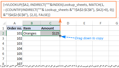
Before diving into VLOOKUP, ensure your data is organized:
- Label Sheets Correctly: Rename your sheets to something clear and descriptive, like ‘SourceData’ and ‘LookupData’.
- Check for Duplicates: Verify that the lookup column in both sheets doesn’t have duplicate values. VLOOKUP returns the first match.
- Ensure Consistent Data Format: Make sure that the data type in the lookup columns (e.g., numbers, dates, or text) matches across sheets.
📌 Note: Organize your data before using VLOOKUP to minimize errors. Use filters or sort functions to double-check your data arrangement.
Step 2: Understand VLOOKUP Syntax

VLOOKUP stands for Vertical Lookup. Its syntax is:
VLOOKUP(lookup_value, table_array, col_index_num, [range_lookup])
- lookup_value: The value you’re searching for.
- table_array: The range containing the lookup table. This is where you need to reference another sheet.
- col_index_num: The column number in the lookup table from which to pull the return value.
- range_lookup: TRUE or FALSE, where TRUE allows an approximate match, and FALSE requires an exact match.
Step 3: Reference Data from Another Sheet
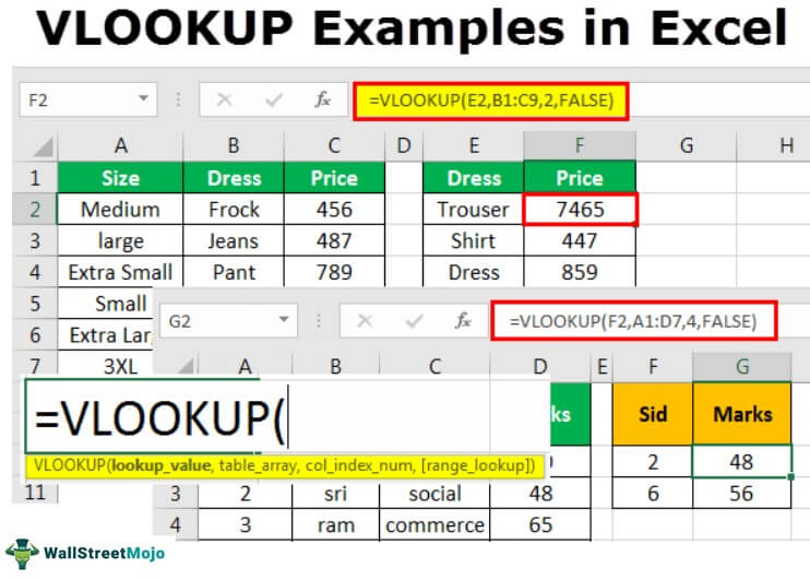
When referencing data from another sheet, adjust the table_array part of VLOOKUP as follows:
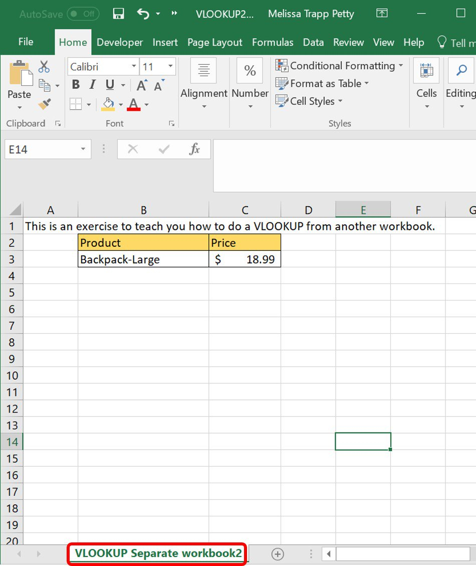
- Go to the sheet where you want to put the VLOOKUP function.
- Type the formula, but replace the standard cell range with a reference to the other sheet, like this:
‘SourceData’!A1:D100instead ofA1:D100.
Here’s an example:
=VLOOKUP(A2,‘SourceData’!A1:D100,4,FALSE)
🔍 Note: Double-check the sheet names and ensure there are no typos. Excel is very particular about syntax when referencing external sheets.
Step 4: Handle Errors and Data Mismatches
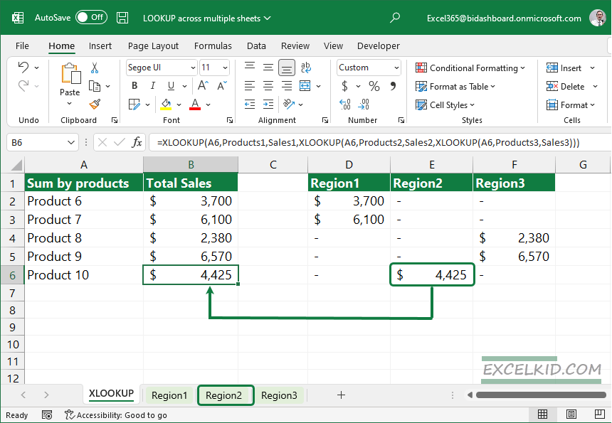
Excel might return errors like #N/A (Not Available) if the lookup value isn’t found, or if there are mismatches in the data:
- Using IFERROR: Wrap your VLOOKUP with IFERROR to display a custom message or handle errors gracefully.
=IFERROR(VLOOKUP(A2,‘SourceData’!A1:D100,4,FALSE),“Value not found”) - Case Sensitivity: VLOOKUP isn’t case-sensitive, but if this is an issue, convert the text to a common case first.
Step 5: Implement and Test

Now that you’ve structured the VLOOKUP formula, implement it:
- Enter the VLOOKUP formula in the cell where you want the matched result to appear.
- Check if the data pulls correctly by looking at a few known matches and verifying the accuracy.
- Drag or copy the formula down if you’re applying it to multiple rows.
In this way, VLOOKUP will help you work efficiently across multiple sheets, providing a seamless experience in data management.
Following these steps ensures that you can harness the power of VLOOKUP across two Excel sheets, making data integration and analysis much smoother and more effective. Understanding the nuances of data organization, formula syntax, error handling, and testing are key to mastering this function.
Can VLOOKUP handle multiple criteria?
+
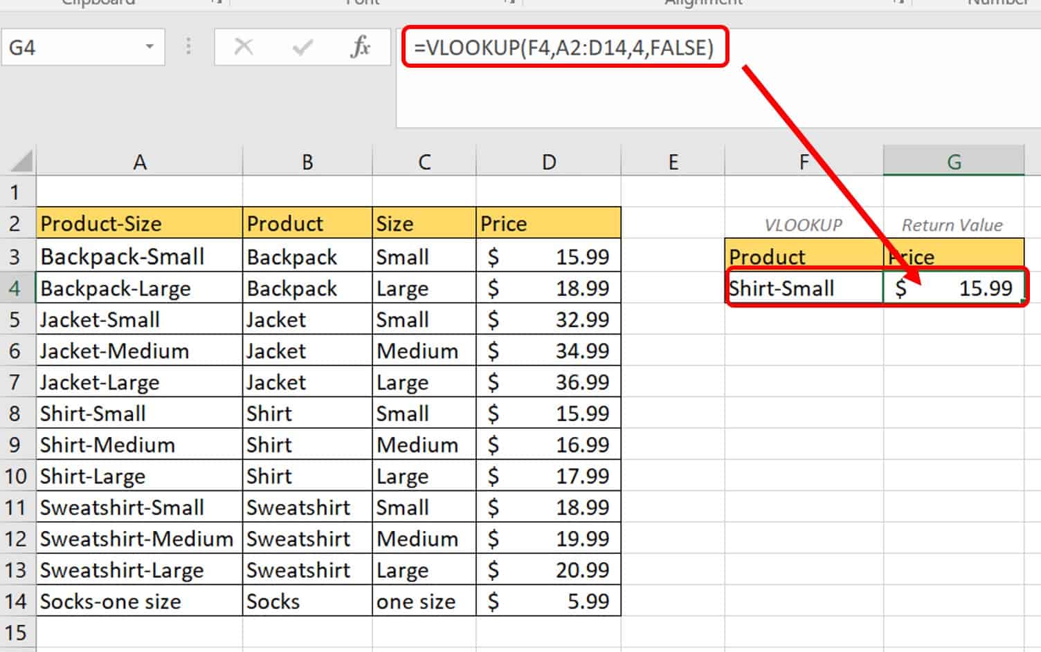
While VLOOKUP itself cannot handle multiple criteria natively, you can use helper columns or functions like INDEX-MATCH to achieve this.
What if my lookup range changes dynamically?
+
You can use named ranges or OFFSET to dynamically adjust the range VLOOKUP searches within.
How do I avoid errors from typos or leading spaces in data?
+
Use the TRIM function to remove extra spaces and the EXACT function to ensure no typos, or consider case sensitivity.