5 Simple Steps for VLOOKUP Between Sheets in Excel 2010

Using VLOOKUP to fetch data between different sheets in Excel can significantly boost productivity when you are dealing with large datasets. This tutorial will guide you through the process of setting up a VLOOKUP formula to work across multiple sheets within an Excel workbook, focusing on the functionality available in Excel 2010.
Step 1: Understand Your Data Layout

Before diving into the formula, ensure you understand how your data is structured:
- Source Sheet: The sheet containing the lookup values you want to match.
- Target Sheet: The sheet where you want the results to appear.
- Identify the common unique key in both sheets for the lookup operation.
Step 2: Prepare the VLOOKUP Formula

To create a VLOOKUP that pulls data from another sheet, you’ll need to reference the external sheet in your formula. Here is the basic structure:
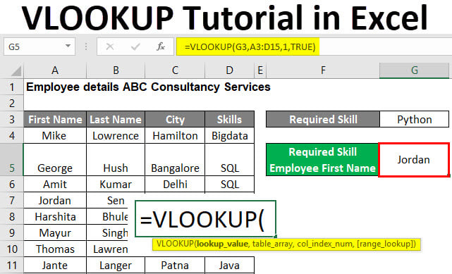
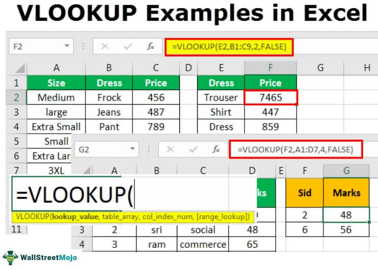
=VLOOKUP(lookup_value, Table_Array, col_index_num, [range_lookup])
lookup_value:This is the cell reference in the target sheet containing the value you want to find in the source sheet.Table_Array:This should point to the range in the source sheet where the lookup will be performed.col_index_num:Indicates which column in the table array to return the value from.range_lookup:Specify FALSE for an exact match, or TRUE for approximate.
Step 3: Construct the VLOOKUP Across Sheets

Assuming your data looks something like this:
- Source sheet name is ‘Products’ with the lookup data starting at A2:D100.
- Target sheet name is ‘Sales’ and you want to insert the VLOOKUP in cell B2.
Here’s how you would write the formula:
=VLOOKUP(A2,Products!A2:D100,3,FALSE)
📝 Note: Make sure the target sheet has the same unique key in the same column as the source sheet for accurate results.
Step 4: Copy the Formula

After inserting the formula in one cell, you can:
- Double-click the fill handle to automatically fill the column down if the values in the adjacent column extend down similarly.
- Or, click and drag the fill handle down to the last row you need the formula in.
Step 5: Test and Verify

Once your VLOOKUP formula is in place:
- Check for errors such as #N/A which indicates the lookup value wasn’t found.
- Ensure all expected matches are returned correctly.
- Consider using IFERROR to handle errors gracefully:
=IFERROR(VLOOKUP(A2,Products!A2:D100,3,FALSE),"No match")
💡 Note: Excel's error values can be useful for debugging, but for a production environment, you might want to display a user-friendly message or blank cells instead.
In summary, mastering the use of VLOOKUP between sheets in Excel 2010 involves understanding your data layout, constructing the VLOOKUP formula correctly, ensuring cross-sheet references are accurate, and thoroughly testing your results. This technique saves time and helps in maintaining data integrity across sheets. Regular checks and maintenance of your lookup formulas can keep your data analysis accurate and efficient.
Can VLOOKUP work with sheets from different workbooks?

+
Yes, but you need to reference the other workbook in the formula. Ensure both workbooks are open, and then include the workbook name in single quotes, an exclamation mark, and the range (e.g., ‘WorkbookName.xlsx’!SheetName!A1:D100).
What can I do if my VLOOKUP is too slow?

+
Consider using Excel’s INDEX/MATCH function instead, which can be faster for large datasets. Also, optimizing your data structure by reducing the lookup range or using named ranges can improve performance.
How can I debug a VLOOKUP that returns incorrect results?

+
Check the data format of your lookup and return values, make sure there are no spaces or hidden characters, and verify that your lookup range is sorted if using TRUE for approximate match.
What’s the difference between an exact and approximate match in VLOOKUP?

+
An exact match (using FALSE) finds an exact value, while an approximate match (using TRUE) looks for the next largest value that is less than or equal to the lookup value, which can be useful for finding thresholds or rates.