5 Easy Ways to Use VLOOKUP Across Two Excel Sheets

Ever found yourself dealing with a multitude of data across different Excel sheets and wished you had a magic wand to connect and pull information between them? Well, consider VLOOKUP as your Excel wizard. This function is highly useful when working with large datasets or when you need to retrieve values based on specific criteria. Here are five straightforward methods to master VLOOKUP across two or more sheets, making your data analysis in Excel a breeze.
Understanding VLOOKUP


Before diving into how to use VLOOKUP across sheets, it’s vital to understand its basic functionality:
- Function Syntax: VLOOKUP(lookup_value, table_array, col_index_num, [range_lookup])
- The lookup_value is the value you want to find.
- table_array is where the function looks for the lookup_value.
- col_index_num tells Excel in which column of the table_array to return the value from.
- range_lookup is an optional parameter for finding an exact or approximate match.
Method 1: Using Sheet References

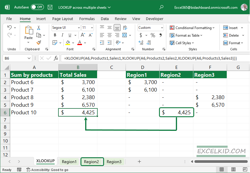
The simplest way to use VLOOKUP across two sheets is by referencing the table directly from another sheet:
=VLOOKUP(A2,Sheet2!A2:C100,2,FALSE)
💡 Note: Remember to use absolute references (A2:C100) when specifying the table array to prevent dragging errors.
Method 2: VLOOKUP with Named Ranges

For a cleaner approach, define named ranges for your table arrays:
- Select the range in the second sheet and give it a name (e.g., ‘DataSheet2’).
- Use this named range in your VLOOKUP formula:
=VLOOKUP(A2,DataSheet2,2,FALSE)
This method not only simplifies your formulas but also makes them more readable and less prone to errors.
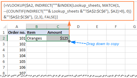
Method 3: Combining VLOOKUP with INDIRECT

If you’re looking to make your VLOOKUP formulas more dynamic, use the INDIRECT function:
=VLOOKUP(A2,INDIRECT(“‘Sheet” & A1 & “’A2:C100”),2,FALSE)
Here, A1 could be a cell containing the name or number of the sheet you want to lookup from. This technique is excellent for user-controlled lookups or when dealing with multiple sheets.
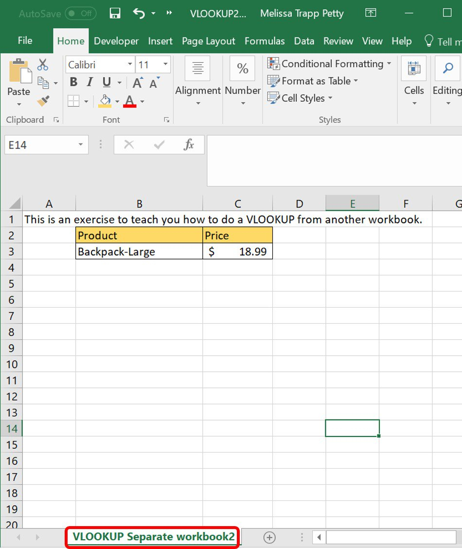
Method 4: VLOOKUP with Data from Different Workbooks

VLOOKUP isn’t limited to a single workbook. Here’s how you can pull data across workbooks:
=VLOOKUP(A2,‘[Data Workbook.xlsx]Sheet2’!A2:C100,2,FALSE)
💡 Note: Keep the external workbook open while working on this. If it’s closed, Excel might prompt you to open it when you open the file containing the formula.
Method 5: Advanced VLOOKUP with Array Formulas

If your data spreads across multiple columns or rows and you need to pull data from different parts of the sheets, an array formula with VLOOKUP can help:
=VLOOKUP(A2,{Sheet2!A2:A100,Sheet2!D2:D100},2,FALSE)
After typing the formula, press Ctrl + Shift + Enter to create an array formula. This allows you to look up across non-adjacent columns within the same sheet.
Summing Up Key Takeaways

Throughout this guide, we’ve covered several methods to use VLOOKUP across multiple Excel sheets, each suited for different data scenarios:
- Sheet References: Simple and direct approach for static data.
- Named Ranges: Enhances formula readability and manageability.
- INDIRECT: Provides dynamic control over data lookup.
- Across Workbooks: Enables data integration from different sources.
- Array Formulas: For handling complex or scattered data.
These techniques empower you to handle datasets efficiently, saving time and reducing errors. Whether you’re managing sales records, inventory, or customer data, these VLOOKUP methods will streamline your workflow.
What if I get a #N/A error with VLOOKUP?

+
This error occurs when VLOOKUP can’t find the lookup value. Ensure the value exists in the first column of the table array, or check for spaces or typos.
How can I use VLOOKUP to search from right to left?

+
VLOOKUP can’t look from right to left; for this, you would need to use INDEX and MATCH functions instead.
Can VLOOKUP work with merged cells?

+
Yes, but ensure that the lookup column or range you’re using doesn’t have merged cells as this can throw off the VLOOKUP function.