Mastering VLOOKUP: Excel's Sheet Linking Guide
Ever wondered how to efficiently connect and manage data across different Excel sheets? The VLOOKUP function is your answer. Excel's dynamic capabilities make handling large data sets both effective and straightforward, reducing time and errors significantly.
What is VLOOKUP?
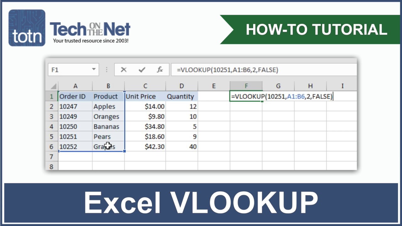
VLOOKUP stands for Vertical Lookup—a function that searches for a value in the first column of a table and retrieves a corresponding value from another column in the same row. This is particularly useful when you need to retrieve information from a separate but related dataset or from a different worksheet.

Why Use VLOOKUP?
- Link Sheets: Link sheets together to keep your workbook organized and make data manipulation seamless.
- Save Time: Automate data retrieval to reduce manual searches and boost efficiency.
- Avoid Errors: Minimize the risk of human errors in data entry by linking directly to the source.
- Improve Scalability: Manage larger datasets with ease as VLOOKUP helps in linking sheets in a scalable way.
How Does VLOOKUP Work?

Here’s how VLOOKUP operates in simple terms:
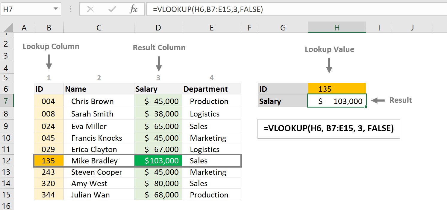
- It searches for a lookup value in the first column of the specified table array.
- Upon finding the value, it retrieves data from another column in the same row as specified by the column index number.
- The range lookup argument lets you define whether you need an exact or approximate match.
Setting Up VLOOKUP in Excel

To set up VLOOKUP:
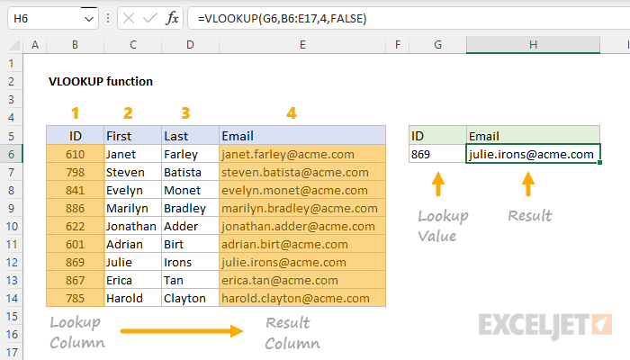
- Ensure a Lookup Value: This is the value you want to look up in another sheet or table.
- Identify the Table Array: This is the range of cells containing the data to search. Remember, the lookup value must be in the first column.
- Set Column Index Number: This tells VLOOKUP which column to pull data from.
- Choose Range Lookup: Either TRUE for an approximate match or FALSE for an exact match.
The formula structure looks like this:
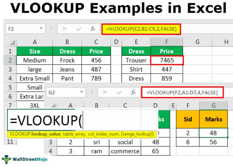
VLOOKUP(lookup_value, table_array, col_index_num, [range_lookup])
✨ Note: If your lookup value doesn't exist in the first column, VLOOKUP will return an error.
Step-by-Step Guide to Linking Sheets with VLOOKUP
- Create Source and Destination Sheets: Make one sheet with the primary data and another where you want to fetch the data. For example, one sheet could be named ‘Sales Data’ and the other ‘Summary Report’.
- Enter the Lookup Value: In the Summary Report, enter or select the value you want to look up in the Sales Data. Suppose it’s the product name or ID.
- Write the VLOOKUP Formula: In a cell of the Summary Report, enter the VLOOKUP function as follows:
VLOOKUP(lookup_value, SalesData!A2:D50, 2, FALSE)
- lookup_value: The cell where the product name or ID is located. - SalesData!A2:D50: The range in the source sheet where the lookup will be performed. - 2: The column number in the Sales Data sheet where the data to be retrieved is. - FALSE: For an exact match. - Copy and Adjust: Copy the formula down or across to apply to other data points.
Advanced Techniques

- Using Named Ranges: Simplify your formulas by using named ranges. For instance, naming the Sales Data range as ‘SalesRange’ reduces the formula to:
VLOOKUP(lookup_value, SalesRange, 2, FALSE)
- Nested VLOOKUP: Perform lookups within lookups to retrieve complex data relationships.
- Dynamic Column Index**: Use the
MATCHfunction to dynamically adjust the column index number.
🔍 Note: For large datasets, consider using INDEX-MATCH as an alternative for better performance.
Common VLOOKUP Mistakes and How to Fix Them

- Incorrect Range: Ensure the lookup value is in the first column of your table array.
- Data Format Mismatch: Make sure the data format in the lookup column matches the lookup value’s format.
- Column Index Errors: Double-check your column index number; it should match the column you’re retrieving data from.
- Case Sensitivity: VLOOKUP is not case-sensitive, but for case-sensitive searches, consider using an alternative like
EXACTfunction.
In this extensive guide, we've explored the power of VLOOKUP to effectively link data across multiple Excel sheets. By understanding how VLOOKUP works, setting it up correctly, and avoiding common pitfalls, you can significantly enhance your data management capabilities. Remember to leverage named ranges and consider dynamic column indexes for more advanced usage, making your data manipulation not just efficient but also highly flexible.
What is the fastest way to learn VLOOKUP?

+
The quickest path to mastering VLOOKUP involves practicing with real datasets, watching tutorials, and using online Excel courses tailored for VLOOKUP.
Can VLOOKUP return multiple values?

+
VLOOKUP itself returns only one value. However, you can use array formulas or combine it with other functions like IFERROR to fetch multiple values.
What happens if the lookup value is not found?
+
VLOOKUP will return an #N/A error if the lookup value does not exist in the first column of the table array.