Mastering VLOOKUP: Link Two Excel Sheets Effortlessly

The VLOOKUP function stands as a cornerstone for anyone working with data in Excel. For analysts, data scientists, or anyone managing information, understanding how to effectively link two Excel sheets can transform the way they handle and analyze data. In this post, we'll delve deep into the VLOOKUP function, illustrating how it can be used to link sheets with ease, and provide practical examples to ensure you can implement this in your daily tasks. Whether you're a beginner or looking to refresh your Excel skills, let's explore how VLOOKUP can streamline your data management.
Understanding VLOOKUP: The Basics

Before we dive into linking sheets, let’s understand what VLOOKUP does:
- VLOOKUP stands for Vertical Lookup, meaning it searches for a value in the first column of a specified table and then returns a value from the same row in a column you specify.
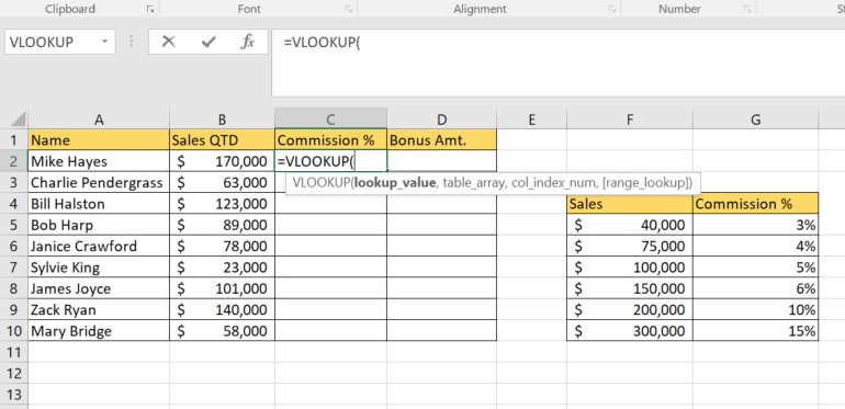
- The syntax of VLOOKUP is:
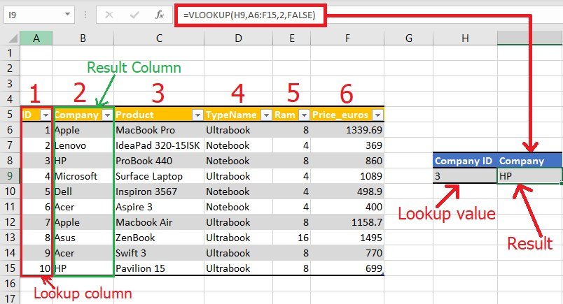
VLOOKUP(lookup_value, table_array, col_index_num, [range_lookup]) - lookup_value: The value you want to find.
- table_array: The range of cells that contains the data.
- col_index_num: The column number in the table from which to retrieve the value.
- range_lookup: A boolean to find an exact match (FALSE) or approximate match (TRUE).
How to Link Two Excel Sheets Using VLOOKUP

Linking two Excel sheets with VLOOKUP involves the following steps:
Step 1: Prepare Your Sheets

- Ensure that there is a common identifier between your sheets. This could be an ID, name, or any unique key.
Step 2: Select the VLOOKUP Range

- In the sheet where you want to add data from another sheet, decide where you’ll apply the VLOOKUP function.
- Select the cell where you want to insert the formula.
Step 3: Construct the VLOOKUP Formula

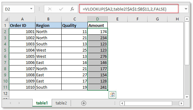
To link two sheets, your formula will look something like this:
VLOOKUP(A2, Sheet2!A:B, 2, FALSE)
- Assuming A2 has the lookup value.
- ‘Sheet2!A:B’ is the range from another sheet where column A is the lookup column, and column B contains the data to retrieve.
- ‘2’ specifies the column number in Sheet2 from which to pull the data.
- ‘FALSE’ ensures an exact match.
Step 4: Adjust for Different Workbooks

- If you’re linking sheets from different Excel workbooks, your formula will change slightly:
VLOOKUP(A2, ‘[WorkBookName]Sheet2’!A:B, 2, FALSE)🔍 Note: Make sure the workbook from which you’re referencing data is open or Excel might return an error.
Real-Life Example

Imagine you manage a sales database across two sheets:
- SalesData: Contains customer names, order numbers, and dates of purchase.
- CustomerInfo: Contains customer names and detailed information like contact details, customer ID, etc.
To link the detailed customer info to the sales data:
- Select the cell next to the customer name in SalesData (let’s say cell B2).
- Enter the following VLOOKUP formula:
=VLOOKUP(A2, CustomerInfo!A2:D100, 2, FALSE)- Here, A2 is the customer name in SalesData, and we’re looking for it in CustomerInfo, pulling data from column 2 (customer ID).
- Drag down to apply the formula to all relevant rows.
📌 Note: Always ensure the columns referenced in your VLOOKUP formula are stable, and it's a good practice to name ranges or use absolute cell references.
Troubleshooting Common VLOOKUP Errors

Here are some common issues you might encounter:
- #N/A Error: The lookup value isn’t found, or you’ve set FALSE for an exact match when the value doesn’t exist.
- #REF! Error: The formula refers to an invalid cell or range.
- Incorrect Results: This might happen if the table array isn’t sorted properly for approximate matches or if you’ve selected the wrong column index.
In wrapping up this exploration of VLOOKUP for linking two Excel sheets, we've covered the function's core mechanics, its application in real-world scenarios, and potential pitfalls to avoid. By mastering VLOOKUP, you're not just connecting data; you're enhancing the efficiency of your data management tasks, which can lead to better decision-making and analysis. Remember, practice is key. The more you work with VLOOKUP, the more intuitive it becomes, allowing you to connect data from different sources seamlessly.
What is VLOOKUP’s limitation in terms of search direction?

+
VLOOKUP only searches from left to right. If you need to look up from right to left, you must use INDEX and MATCH or other lookup functions.
Can VLOOKUP be used with wildcards?

+
Yes, VLOOKUP supports wildcards when the range_lookup argument is set to FALSE. You can use * for multiple characters or ? for a single character.
Is it possible to perform VLOOKUP on multiple criteria?

+
Not directly with VLOOKUP. You’ll need to use helper columns or array formulas, or consider using INDEX and MATCH functions for this task.
How does VLOOKUP handle duplicate values in the first column?

+
VLOOKUP will return the value associated with the first occurrence of the lookup value in the table array when exact match is requested.