5 Ways to Master Pivot Tables in Excel Easily

Are you overwhelmed by the vast amount of data that you need to analyze in Excel? If so, you're not alone. Excel is a powerful tool with many features designed to simplify data management, and one of its most useful capabilities is the pivot table. This tool can help transform your messy, unstructured data into insightful, summarized reports at the click of a button. Here are five straightforward ways to master pivot tables in Excel, allowing you to analyze and report data more efficiently.
1. Understand the Basics of Pivot Tables

Before you dive into creating complex pivot tables, ensure you have a solid grasp of the basics:
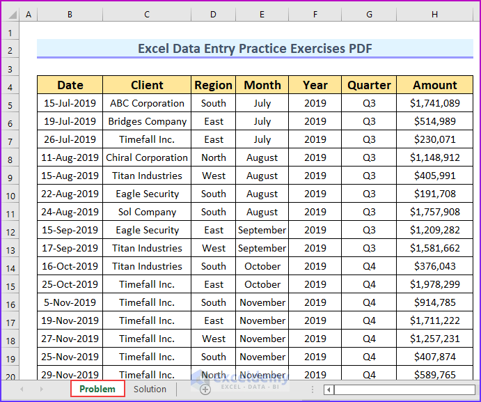
- Data Source: Pivot tables rely on a well-structured dataset. Ensure your data is in a tabular format with no blank rows or columns.
- Row Labels: These are the categories by which you want to slice your data. For instance, if you’re analyzing sales by region, regions would be your row labels.
- Column Labels: Similar to row labels but arranged horizontally, often used for summarizing data by time periods or different product lines.
- Values: This is where the numbers come into play. You decide how these should be displayed, such as sum, average, or count.
2. Build Your First Pivot Table

Here’s a step-by-step guide to creating your first pivot table:
- Select the range of data you want to analyze.
- Go to the Insert tab, then click on PivotTable.
- Choose where you want the PivotTable to be placed. It can be on a new worksheet or an existing one.
- The PivotTable Field List appears on the right side of your screen. Drag fields into the four areas: Filters, Columns, Rows, and Values.
💡 Note: Remember that the success of your pivot table depends heavily on how well your data is organized.
3. Use Calculated Fields and Items

One of the advanced features of pivot tables is the ability to create custom calculations:
- Calculated Fields: Add new data derived from existing data fields. For example, you could add a field to calculate profit by subtracting costs from sales.
- Calculated Items: These allow you to perform calculations on specific items within a field. For instance, calculating the total sales for two specific products from your data.
To add a calculated field:
- Click anywhere inside the pivot table to activate the PivotTable Tools on the Ribbon.
- Go to Analyze tab > Fields, Items, & Sets > Calculated Field.
- Type in the formula and name your field.
| Formula Example | Application |
|---|---|
| =Sales-Cost | Calculates Profit |
| =Sales*0.10 | Calculates 10% Commission |

💡 Note: Before adding a calculated field, ensure that your original data contains all necessary components for the formula.
4. Grouping Data for Better Analysis

Grouping is a powerful pivot table feature:
- Date Grouping: You can group dates by months, quarters, or years, which is ideal for trend analysis.
- Number Grouping: Group numerical data into ranges. This could be useful for age ranges or salary brackets.
- Custom Grouping: For categories not directly in your data, like combining similar products into a group.
To group data:
- Right-click on any data point in the pivot table and select Group.
- Choose the grouping options based on your data type (dates, numbers, etc.).
5. Leverage Pivot Charts for Visual Impact

Pivot charts allow you to visualize your pivot table data:
- Go to the Analyze tab > PivotChart, and select a chart type that best represents your data.
- Adjust the chart elements as needed to highlight trends, comparisons, or patterns.
- Use filters to dynamically change the data being visualized.
To wrap up, mastering pivot tables in Excel can significantly enhance your data analysis capabilities. From understanding the basics to exploring advanced features like calculated fields and charts, pivot tables are an indispensable tool for any data analyst. They help you make sense of large datasets by summarizing and presenting them in meaningful ways, which can be crucial for decision-making in various business scenarios.
Can I add data to a pivot table after it’s created?

+
Yes, you can easily update your pivot table by refreshing it to include new data. Right-click inside the pivot table and select Refresh.
What if my data has many empty cells?

+
Excel handles empty cells by treating them as zero or blank in most cases. However, for accurate analysis, fill or delete these cells as needed.
Can I show percentages in a pivot table?

+
Yes, you can. Click on the value field, go to Show Values As, and select % of Total or another percentage option.