Excel Lookup Guide: Master VLOOKUP in Minutes

Welcome to our Excel Lookup Guide, where mastering the art of VLOOKUP has never been easier or more accessible. Whether you're a beginner dipping your toes into Excel's vast capabilities or an intermediate user looking to refine your data analysis skills, this guide will walk you through the intricacies of VLOOKUP, providing you with the knowledge to use this powerful function effectively in your spreadsheets.
What is VLOOKUP?
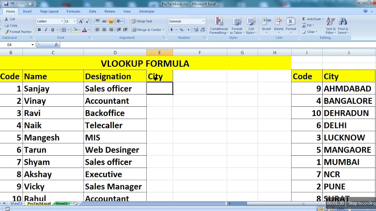
VLOOKUP, which stands for Vertical Lookup, is an Excel function that allows you to search for a value in the first column of a table and return a value in the same row from another column. Here are the basics you need to know:
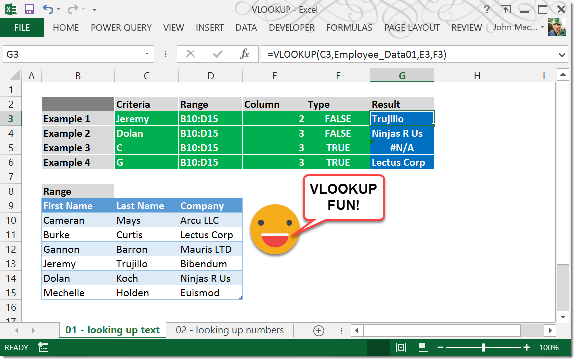
- Function Syntax: =VLOOKUP(lookup_value, table_array, col_index_num, [range_lookup])
- lookup_value: The value you want to search for.
- table_array: The range containing the data. The lookup_value must be in the first column of this range.
- col_index_num: The column number in the table_array from which to retrieve the value.
- range_lookup: (Optional) TRUE for an approximate match or FALSE for an exact match. Defaults to TRUE if omitted.
Understanding VLOOKUP Components

Before diving into VLOOKUP, let’s break down its components to understand how it works:
| Component | Description |
|---|---|
| Lookup Value | The reference point or key you're searching for within your table. |
| Table Array | The range of cells that contains the data. VLOOKUP searches the first column of this array for the lookup_value. |
| Column Index Number | The position of the column from which you want VLOOKUP to return a value. The first column is 1, the second is 2, and so on. |
| Range Lookup | Determines whether you want an exact match (FALSE) or an approximate match (TRUE or omitted). |

Steps to Use VLOOKUP in Excel
Let’s go through the step-by-step process of implementing VLOOKUP in your Excel worksheets:
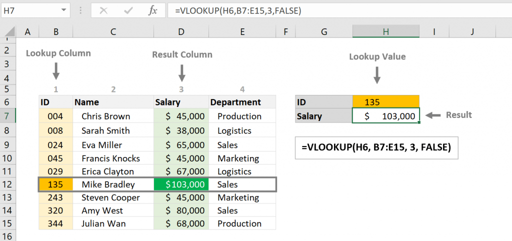
- Prepare Your Data: Ensure your data is organized with the lookup values in the first column of your table array.
- Enter the Formula: Click where you want the result to appear and type or paste the VLOOKUP formula.
- Set the Lookup Value: Specify the cell that contains the value you want to look up.
- Define the Table Array: Select the range where your data is stored, making sure the lookup column is the first column.
- Specify the Column Index Number: Enter the number of the column where the result should be retrieved from.
- Decide on Range Lookup: Choose FALSE for exact matches or leave it blank/TRUE for approximate matches.
⚠️ Note: VLOOKUP performs better with sorted data when using approximate matches. For exact matches, sorting is not required, but it can improve performance.
Common VLOOKUP Mistakes and How to Avoid Them

Here are some pitfalls you might encounter and how to steer clear of them:
- Lookup Value Not in the First Column: VLOOKUP only searches the first column of the table array. Make sure your lookup values are indeed in the first column.
- Incorrect Column Index Number: Double-check the column index to ensure it corresponds to the column you want to retrieve data from.
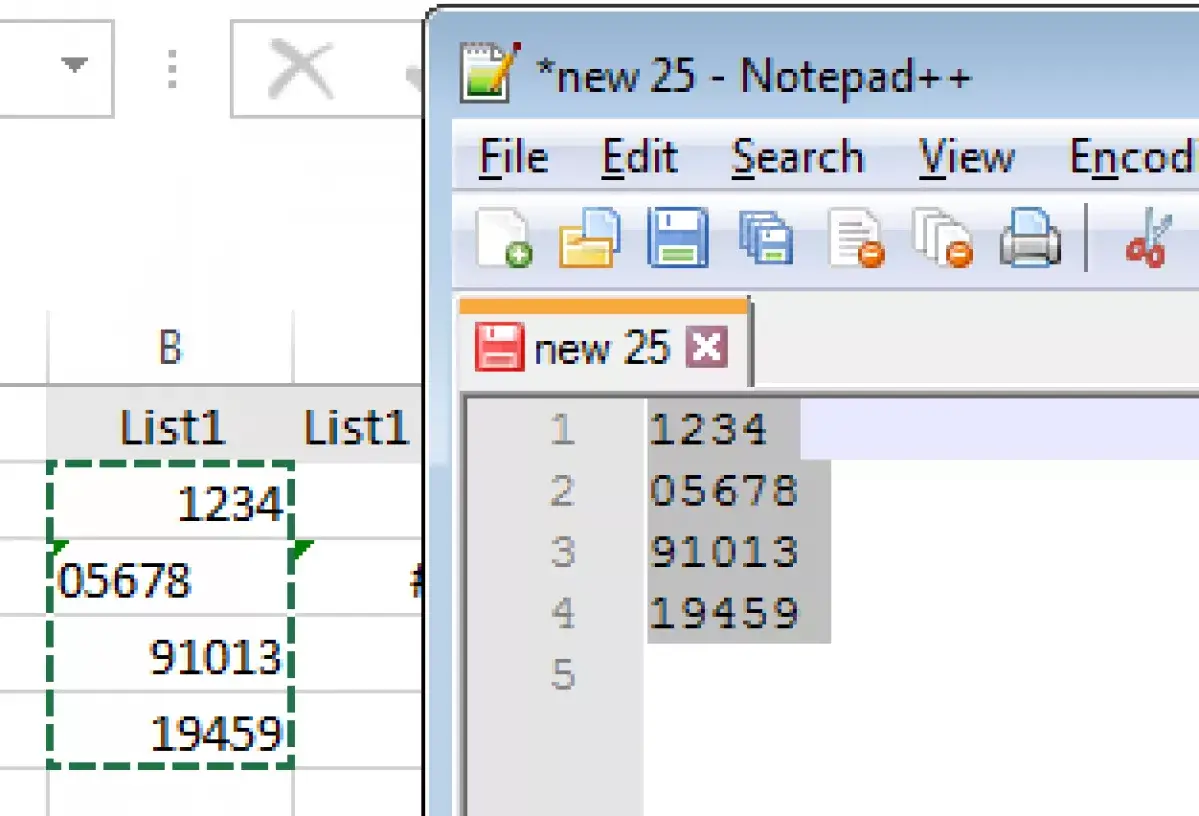
- Data Types Mismatch: Ensure the data type (text, number, etc.) of the lookup value matches the type in your table.
- Missing or Incorrect Range Lookup Argument: If you’re looking for an exact match, always set the range lookup to FALSE.
Advanced VLOOKUP Techniques
While VLOOKUP is straightforward, here are some advanced techniques to enhance its functionality:
Using Named Ranges
Named ranges can make your formulas cleaner and easier to read:
=VLOOKUP(A2, ProductList, 3, FALSE)
Nested VLOOKUPs

You can nest VLOOKUP functions within other functions like IF or CHOOSE to handle more complex data scenarios:
=IF(VLOOKUP(A2,Table1,4,FALSE)=“Yes”, VLOOKUP(A2,Table2,2,FALSE), “Not Applicable”)
VLOOKUP with Wildcards

If you need to look for partial matches, wildcards can be useful:
- Asterisk (*): Represents any number of characters.
- Question Mark (?): Represents one character.
VLOOKUP with Dynamic Table Array

Use dynamic references with MATCH function to adjust the table array based on criteria:
=VLOOKUP(A2, OFFSET(B2,0,0,MATCH(“XYZ”,A:A,0),4), 4, FALSE)
With these techniques, you can significantly expand VLOOKUP's capabilities in your data analysis.
VLOOKUP Alternatives

While VLOOKUP is powerful, there are situations where other functions might be more suitable:
- HLOOKUP: For horizontal lookups when your data is laid out row-wise.
- INDEX and MATCH: More flexible, allowing you to look up in both directions and across multiple sheets or workbooks.
- XLOOKUP: (Available in newer versions of Excel) Overcomes many limitations of VLOOKUP by allowing reverse and multiple criteria searches.
By the end of this journey, you'll not only understand the core function of VLOOKUP but also how to leverage its potential to transform the way you work with data in Excel.
What is the main purpose of VLOOKUP in Excel?
+
The primary purpose of VLOOKUP is to look up a value in the first column of a table and return a value from another column in the same row.
Can VLOOKUP search to the left?

+
No, VLOOKUP cannot natively search to the left. It always looks for the value in the leftmost column of the table array. For searching to the left, you would typically use a combination of INDEX and MATCH functions.
How does approximate matching work in VLOOKUP?

+
With approximate matching (TRUE), VLOOKUP finds the largest value less than or equal to the lookup_value when an exact match isn’t available. This is useful for tiered pricing or grading systems, but your data should be sorted in ascending order for accurate results.