VLOOKUP Guide: Matching Data Across Two Excel Sheets

Understanding VLOOKUP: A Key Excel Function for Data Analysis

When working with large datasets in Microsoft Excel, one of the most powerful tools at your disposal is the VLOOKUP function. VLOOKUP, short for 'Vertical Lookup,' allows you to search for a value in the first column of a table and return a value in the same row from another column. This function becomes indispensable when you need to match data across two or more sheets efficiently.
How Does VLOOKUP Work?

VLOOKUP follows a simple yet effective structure:
- Lookup Value: The value you're searching for within the first column of a table array.
- Table Array: The range of cells that contains the data. This should include the lookup column and the column from which you want to retrieve data.
- Column Index Number: The column number in the table array from which you want to retrieve the value, counting from the leftmost column.
- Range Lookup: This is a logical value: TRUE for an approximate match or FALSE for an exact match.
Step-by-Step Guide to Using VLOOKUP

Setting Up Your Data

Before diving into VLOOKUP, ensure your data is:
- Organized with headers.
- Formatted correctly (no merged cells in the lookup column).
- The lookup column is the first column in your table array.
Basic VLOOKUP Syntax

The syntax for VLOOKUP looks like this:
VLOOKUP(lookup_value, table_array, col_index_num, [range_lookup])
Practical Examples

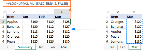
Let's go through two practical examples to understand VLOOKUP in action:
- Example 1: Matching Employee ID to Department
Assume you have two sheets. Sheet 1 contains employee details, and Sheet 2 has department information. You want to add the department names to the employee details sheet.
VLOOKUP(A2, Sheet2!A:B, 2, FALSE)🔍 Note: Here, A2 refers to the employee ID in Sheet 1, and the second parameter points to the department table in Sheet 2.
- Example 2: Finding Product Price
In this scenario, you have a list of product IDs and need to find their corresponding prices from a separate price list sheet.
VLOOKUP(ProductID, Prices!$A$2:$C$100, 3, FALSE)Here, 'ProductID' is the cell containing the product ID you're looking up, 'Prices!$A$2:$C$100' is the range with product IDs and prices, 3 specifies the third column (the price), and FALSE ensures an exact match.
Important Considerations

When using VLOOKUP, remember:
- Exact matches are generally more reliable than approximate matches unless your data supports approximate lookup.
- If the lookup value is not found, VLOOKUP returns #N/A error.
- VLOOKUP cannot look to the left; it only searches columns to the right of the lookup column.
Tips for Optimizing VLOOKUP

To enhance the performance and accuracy of your VLOOKUP formulas:
- Use named ranges for your table array to make the formula more readable and manageable.
- Sort the lookup column if using an approximate match to avoid errors.
- Consider using
IFERRORto handle #N/A errors gracefully.IFERROR(VLOOKUP(A2, Sheet2!A:B, 2, FALSE), "Not Found")
Alternative to VLOOKUP: INDEX and MATCH

While VLOOKUP is powerful, the combination of INDEX and MATCH functions offers more flexibility:
| Function | VLOOKUP | INDEX and MATCH |
|---|---|---|
| Flexibility | Only searches to the right. | Can search in any direction. |
| Performance | Slower on large datasets. | Generally faster. |
| Maintenance | Difficult if the table changes. | Easier to update if columns change. |

Final Thoughts

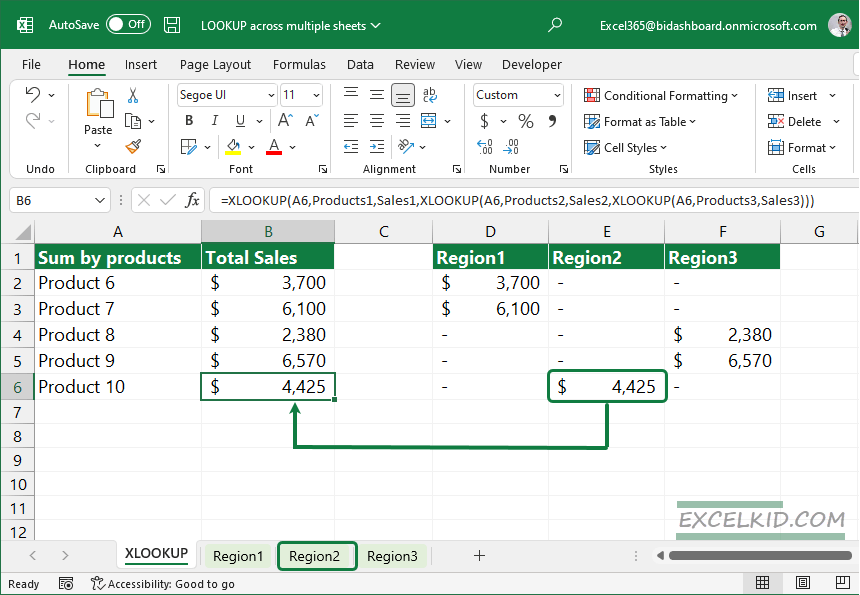
Mastering VLOOKUP opens up numerous possibilities for efficient data analysis in Excel. It streamlines the process of matching and extracting data from large spreadsheets, reducing the time and effort required for manual lookups. Whether you're combining data from multiple sheets or just simplifying complex data sets, VLOOKUP is a tool that can significantly enhance your productivity. Just remember to prepare your data correctly, choose your match type wisely, and consider alternatives like INDEX and MATCH for more advanced scenarios.
What does VLOOKUP do when the lookup value is not found?

+
VLOOKUP returns an #N/A error when it cannot find the specified lookup value in the first column of the table array. This error indicates that there was no exact or approximate match found.
Can VLOOKUP look up data from left to right?

+
No, VLOOKUP is designed to only search columns to the right of the lookup column. If you need to look left, consider using INDEX and MATCH or XLOOKUP in newer versions of Excel.
How can you handle errors in VLOOKUP?

+
You can use the IFERROR function to handle errors gracefully. For example, IFERROR(VLOOKUP(A2, Sheet2!A:B, 2, FALSE), “Not Found”) will return “Not Found” instead of #N/A if the lookup value isn’t found.