VLOOKUP Made Easy: Connect Data Across Excel Sheets

Understanding VLOOKUP

VLOOKUP, short for Vertical Lookup, is one of the most useful functions in Microsoft Excel. It allows users to search for a specific value in a column of data and then return a value from another column in the same row. This is particularly helpful when you have a large dataset split into different sheets or tables, and you need to connect information from these different sources effortlessly. In this comprehensive guide, we will delve into the ins and outs of VLOOKUP to make it an easy and indispensable part of your Excel toolkit.

When to Use VLOOKUP

VLOOKUP is ideal in several scenarios:

• When you need to lookup and retrieve data from a separate table, especially when the table is in another worksheet or workbook.
• When you want to automate data entry by pulling information from a master list.
• When you need to cross-reference information between different datasets for reporting or analysis purposes.

The Syntax of VLOOKUP

The syntax of the VLOOKUP function is straightforward:

VLOOKUP(lookup_value, table_array, col_index_num, [range_lookup])

Here's what each parameter means:

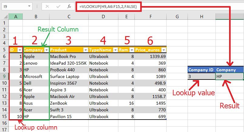
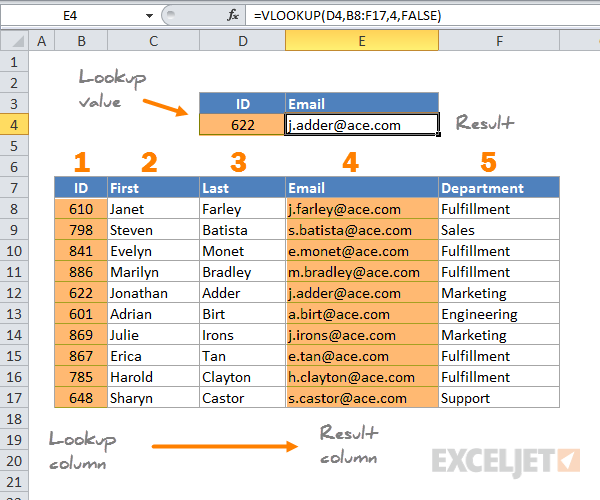
• lookup_value: The value you want to search for in the first column of your table array.
• table_array: The range of cells that contains the data.
• col_index_num: The column number in the table from which to retrieve the value.
• range_lookup: An optional argument; TRUE finds the closest match (if the table isn't sorted, it will give an error), FALSE finds an exact match.

Step-by-Step Guide to Using VLOOKUP

1. Preparing Your Data

Before you can use VLOOKUP, ensure:

• Your data is organized vertically in a table format.
• The first column of the table contains the unique identifier or the lookup values.
• The column with the data you want to return is to the right of the lookup column.

2. Entering the Formula

Follow these steps to enter the VLOOKUP formula:

1. Select the cell where you want the VLOOKUP result to appear.
2. Type in "=VLOOKUP(".
3. Click or type the lookup_value (the value you're looking for).
4. Press the comma key and select your table_array.
5. Enter the col_index_num - the column number from which you want to retrieve the value.
6. Press the comma again and type "TRUE" or "FALSE" for range_lookup.
7. Close the parenthesis and press Enter.

Example:

Let's say you have two sheets:

• Sheet1 with employee IDs and their names.
• Sheet2 with employee IDs and their departments.

You want to know the department for a specific employee ID. Here's how you would set up your VLOOKUP:

=VLOOKUP(A2,Sheet2!A:B,2,FALSE)

Where:

• A2 is the employee ID you want to look up.
• Sheet2!A:B is the range in Sheet2 where IDs and departments are located.
• 2 specifies that you want to retrieve the value from the second column (Department).
• FALSE ensures you get an exact match.

🧩 Note: Always ensure your lookup column in the table_array is the first column. If not, Excel will return an error or the wrong result.

Advanced VLOOKUP Techniques

Using VLOOKUP with Wildcards

VLOOKUP supports wildcard characters like * (any number of characters) and ? (one character). This can be useful for partial matches:

=VLOOKUP("Smi*",A1:B10,2,FALSE)

This formula looks for names starting with "Smi" in column A and returns the corresponding value from column B.

Handling Errors with IFERROR

VLOOKUP can return errors if the lookup value isn't found or if there's an issue with the data. You can wrap your VLOOKUP with IFERROR to return a custom message or a default value:

=IFERROR(VLOOKUP(A2,Sheet2!A:B,2,FALSE),"Not Found")

Dynamic Column Index

Instead of hard-coding the column index number, you can use the MATCH function to dynamically identify the column:

=VLOOKUP(A2,Sheet2!A:D,MATCH(“Department”,Sheet2!A1:D1,0),FALSE)

This formula will locate the column named “Department” in the header row of Sheet2 and return the corresponding value for the employee ID in A2.

In this final wrap-up, VLOOKUP has been demystified and shown to be a powerful tool for connecting data across Excel sheets. By understanding when to use it, mastering its syntax, and learning some advanced techniques, you can greatly enhance your data manipulation capabilities in Excel. Remember to keep your data organized, use VLOOKUP wisely to avoid errors, and always double-check your results for accuracy. With these skills, you're now equipped to manage and analyze large datasets with ease, making your work with Excel much more efficient and insightful.

What does the FALSE argument in VLOOKUP do?

+

Using FALSE as the range_lookup argument in VLOOKUP ensures that Excel searches for an exact match of the lookup value. If an exact match isn’t found, Excel will return an error.

Can VLOOKUP pull data from another workbook?

+

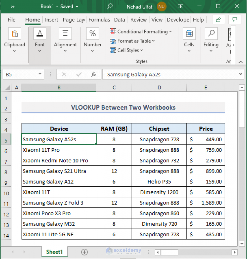
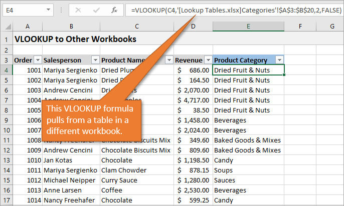
Yes, VLOOKUP can reference data from another workbook. However, the external workbook must be open for VLOOKUP to work; otherwise, it will return an error. The formula would look something like =VLOOKUP(A2,‘[ExternalWorkbook.xlsx]Sheet1’!A:B,2,FALSE).

How can I use VLOOKUP to retrieve multiple columns of data?

+

VLOOKUP by itself only returns one column at a time. To retrieve multiple columns, you can use VLOOKUP in separate columns, or consider using more advanced functions like INDEX/MATCH or the recently introduced XLOOKUP for more flexibility.

What are some common errors when using VLOOKUP?

+

Common VLOOKUP errors include #N/A (value not found), #REF! (column index number is larger than the number of columns in the range), and #VALUE! (data type mismatch or incorrect formula syntax). Ensure your lookup value matches the data type in the lookup column and check your formula for accuracy.