Sheet Reference Magic: Excel Hacks for Efficient Referencing

In the realm of Excel, the ability to create dynamic and efficient data references is not just a luxury; it’s a necessity for anyone looking to streamline their workflow. Whether you’re a financial analyst, a project manager, or a student compiling research data, mastering Excel’s sheet referencing techniques can significantly boost your productivity. Here, we will explore a variety of Excel hacks designed to enhance your data referencing capabilities, ensuring accuracy, speed, and efficiency.
Understanding Excel Sheet References

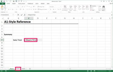
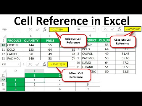
Before diving into the hacks, let's understand the basics of sheet references: - Direct Reference: This involves typing the sheet name followed by an exclamation mark and the cell or range you want to reference, e.g., `Sheet2!A1`. - 3D References: Used when you want to reference the same cell or range across multiple sheets, e.g., `=SUM(Sheet1:Sheet3!A1)`. - Named Ranges: Assigning names to cells or ranges makes references more intuitive, e.g., `=Sales_March`.

Hack 1: Dynamic Sheet References with INDIRECT

The `INDIRECT` function can convert text into cell references, allowing for dynamic referencing: ```excel =INDIRECT("'" & A1 & "'!B2") ``` Here, if cell A1 contains the text "Sheet2", the formula will reference B2 in Sheet2. This method is particularly useful when: - Switching Sheets: If your data frequently changes location, you can simply update the sheet name in one cell rather than rewriting formulas. - Dashboard Creation: Use this to pull data from various sheets into a summary or dashboard sheet dynamically.
🔑 Note: While `INDIRECT` is powerful, it can make your workbook less transparent, potentially increasing the risk of errors if not used judiciously.
Hack 2: Simplify with CHOOSE and MATCH

Combining `CHOOSE` and `MATCH` functions provides an alternative approach for dynamic references: ```excel =CHOOSE(MATCH("Q1", A1:A4, 0), Sheet1!B2, Sheet2!B2, Sheet3!B2, Sheet4!B2) ``` Here: - MATCH finds the position of the quarter you're looking for. - CHOOSE then references the corresponding cell from the matched position. This can be expanded to work with multiple cells: ```excel =CHOOSE(MATCH("Q1", A1:A4, 0), Sheet1!B2:D2, Sheet2!B2:D2, Sheet3!B2:D2, Sheet4!B2:D2) ```
Hack 3: Utilizing the OFFSET Function

`OFFSET` can move from a known reference point, which is helpful for creating dynamic references: ```excel =OFFSET(Sheet1!A1, 1, 2) ``` This formula refers to a cell 1 row down and 2 columns to the right of Sheet1!A1. - Create Rolling Totals: Offset can help in creating totals that move with your data as it grows.
Hack 4: VLOOKUP with Cross-Sheet Referencing

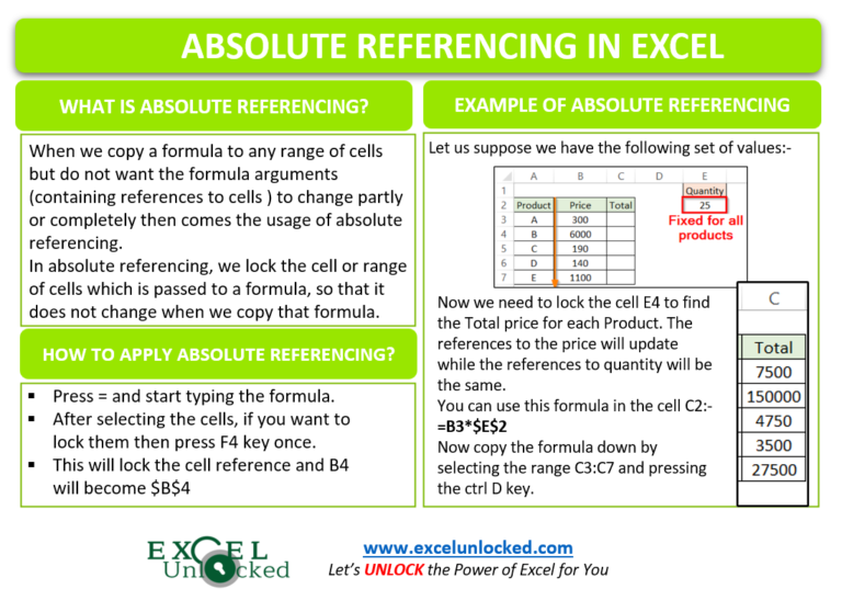
`VLOOKUP` remains a staple for Excel users, but combining it with cross-sheet referencing maximizes its utility: ```excel =VLOOKUP($A$1, Sheet2!$A$1:$B$20, 2, FALSE) ``` This formula: - Searches for the value in A1 from the current sheet within Sheet2!A1:B20. - Returns the value from the second column of that range. For multi-sheet lookups, consider: ```excel =IFERROR(VLOOKUP($A$1, Sheet2!$A$1:$B$20, 2, FALSE), IFERROR(VLOOKUP($A$1, Sheet3!$A$1:$B$20, 2, FALSE), "Not Found")) ```
Hack 5: The Power of Power Query for Advanced Referencing

Power Query (Get & Transform in Excel) allows you to connect to various data sources and perform complex data transformations: - Consolidating Data: Combine data from multiple sheets or workbooks. - Dynamic Update: Automatically update data as it changes in source locations. Here's how you might use Power Query: - Import multiple sheets using From Folder to consolidate data. - Use M Language to create custom functions for complex referencing.
📄 Note: Power Query requires an understanding of its interface and capabilities to fully leverage its potential for referencing.
Hack 6: Macros and VBA for Advanced References

For Excel power users, Visual Basic for Applications (VBA) can automate complex referencing tasks: ```vba Sub DynamicReference() Dim ws As Worksheet Dim cell As Range For Each ws In ThisWorkbook.Worksheets For Each cell In ws.Range("A1:A10") If cell.Value = "Target" Then Debug.Print "Found in " & ws.Name & " at " & cell.Address End If Next cell Next ws End Sub ``` This VBA script searches for the string "Target" across all worksheets, printing its location.
Streamlining Data Management

Efficient sheet referencing in Excel isn’t just about saving time; it’s about maintaining data integrity and making your workflow more resilient to changes:
- Scalability: Techniques like
INDIRECTand Power Query allow for scalability as your data grows or changes structure. - Automation: Macros and functions reduce manual errors and increase productivity.
- Data Integrity: With dynamic references, your data remains accurate even if moved or modified.
By mastering these Excel hacks for sheet referencing, you’ll not only become more proficient with Excel but also unlock new levels of data manipulation that can profoundly impact how you work with information.
How do I make a sheet reference update automatically if I rename the sheet?

+
To make a sheet reference update automatically when renamed, use the INDIRECT function. Ensure the sheet names are dynamically referenced from cells or named ranges, as the formula will pick up the updated name.
What’s the benefit of using named ranges for references?

+
Named ranges make your formulas easier to read and understand, reduce errors when changing references, and improve navigation within Excel. They’re particularly useful when dealing with complex spreadsheets where direct cell references might be confusing or prone to errors.
Can I use these referencing techniques in Google Sheets?

+
Many of these techniques, particularly INDIRECT, CHOOSE, and VLOOKUP, are also applicable in Google Sheets. However, features like Power Query and VBA are specific to Excel, though Google Sheets has its scripting language, Google Apps Script, for automation.