5 Ways to Split Your Excel Sheet Easily

Splitting an Excel sheet can be a vital task for enhancing data organization, improving readability, or segregating different sets of information for various purposes. Whether you're a financial analyst, a marketing manager, or a data enthusiast, knowing how to efficiently split your Excel sheet can streamline your workflow significantly. Here's a detailed guide on five different methods you can use to split your Excel sheet with ease.

1. Use Excel’s Built-In Split Feature

Excel has a straightforward split feature that allows you to view different parts of your worksheet simultaneously.

• Open your Excel workbook.
• Select the cell where you want the split to occur.
• Go to the View tab.
• Click on Split.
• Now, you’ll see vertical and/or horizontal lines appear, allowing you to split the window either vertically, horizontally, or both.

Once split, you can scroll different sections independently. To remove the split, you can either drag the split lines to the edge of the sheet or go back to the View tab and click Split again to turn it off.

2. Freeze Panes for a Fixed Section

Sometimes, instead of splitting, you might want to keep a portion of your sheet visible as you scroll through the rest:

• Navigate to the cell just below where you want to freeze rows or just right of the column you want to freeze.
• Head to the View tab.
• Click on Freeze Panes and choose from:
  • Freeze Top Row
  • Freeze First Column
  • Freeze Panes (to freeze both rows and columns up to the selected cell)

This method doesn’t physically split your sheet but can give the illusion of doing so by keeping parts of it static as you move around.

3. Split Data into Multiple Sheets Using VBA

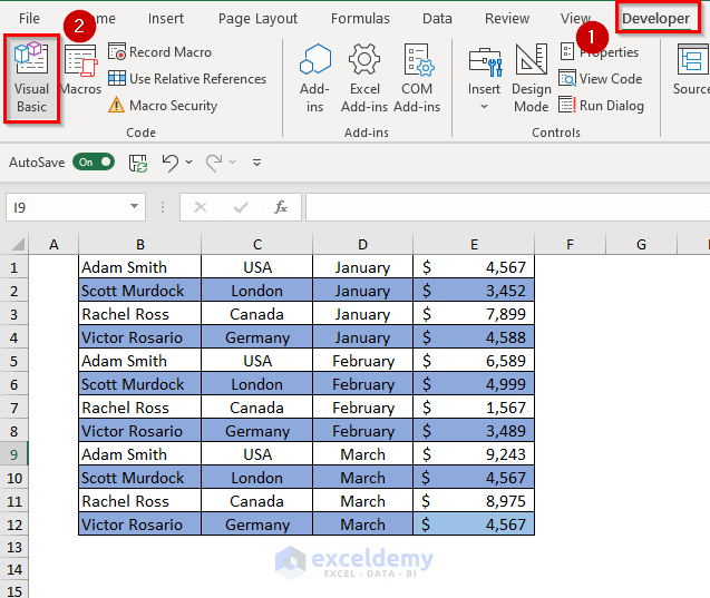
For more complex data manipulation, you might need to split data into entirely new sheets. Here’s a simple VBA script to do just that:

Sub SplitDataIntoNewSheets()
    Dim LastRow As Long
    Dim ws As Worksheet
    Dim NewWs As Worksheet
    Dim i As Long, j As Long

' Determine the last row with data
LastRow = Cells(Rows.Count, 1).End(xlUp).Row

' Loop through rows
For i = 1 To LastRow
    Set NewWs = Sheets.Add(After:=ActiveSheet)
    NewWs.Name = Cells(i, 1).Value ' Assuming first column contains the split criteria
    ' Copy data to the new sheet
    For j = 1 To ActiveSheet.UsedRange.Columns.Count
        NewWs.Cells(1, j).Value = ActiveSheet.Cells(i, j).Value
    Next j
Next i


End Sub

Insert this script into a new VBA module in your workbook and run it to split data based on the values in the first column.

💡 Note: This VBA method requires basic knowledge of Excel macros. Always backup your data before running scripts!

4. Use Advanced Filter to Split Data

The Advanced Filter in Excel can help you split data without writing a single line of code:

• Go to Data tab > Advanced.
• In the ‘Action’ section, select Copy to another location.
• Set your criteria range to filter the data. For example, if you’re filtering by names or categories, this is where you define those.
• Provide the Copy to range (where the filtered data will be copied).
• Optionally, select Unique records only to get unique values.

By setting up an advanced filter, you can split your data based on any criteria you choose into a new location, effectively creating a dynamic data split.

5. Manual Data Division

If your requirements are straightforward or you’re dealing with a small dataset, manual splitting can be the simplest option:

• Highlight the data range you wish to split.
• Right-click on the selection border, choose Copy.
• Navigate to a new sheet or any blank area in your workbook.
• Right-click again and select Paste.
• Repeat the process for other segments of your data.

Manual division might seem basic, but it’s incredibly intuitive for quick and small data reorganizations.

After exploring these methods, you should be well-equipped to handle your Excel data splitting tasks effectively. Each method has its own set of advantages, from simplicity and speed to customization and automation. By choosing the right technique for your specific data needs, you can enhance your productivity and data management significantly. Now, organizing complex data into manageable chunks is as straightforward as ever, allowing you to focus more on analysis and less on the grunt work of data preparation.

What is the difference between splitting and freezing panes in Excel?

+

Splitting divides your Excel window into separate panes for simultaneous viewing of different parts of the same worksheet. Freezing panes keeps rows or columns in view as you scroll through other parts of your data.

Can I split my data based on unique values in a column?

+

Yes, you can use the VBA method described or set up an Advanced Filter with the ‘Unique records only’ option to achieve this.

How can I revert the split or freeze action?

+

Unsplit or unfreeze panes by going to the View tab and clicking Split or Freeze Panes respectively, or by manually dragging the split line back to the edge of the sheet.