5 Easy Ways to Cross-Reference Excel Sheets

In the world of data analysis, Excel remains an indispensable tool. With its powerful capabilities for managing and analyzing vast datasets, Excel can be both a boon and a challenge, especially when dealing with multiple sheets or workbooks. Cross-referencing data between different Excel sheets is a common task that can help ensure accuracy and consistency. In this guide, we'll explore 5 easy ways to cross-reference Excel sheets to streamline your data management processes.
1. Using VLOOKUP Function

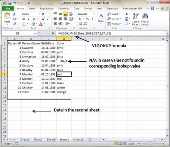
VLOOKUP or Vertical Lookup is probably one of the most widely used functions for cross-referencing in Excel. Here’s how to use it:
- Select the cell where you want the result to appear.
- Enter the formula:
=VLOOKUP(lookup_value, table_array, col_index_num, [range_lookup]) lookup_value: The value you want to search for.table_array: The range of cells that contains the data, from the first column to the last column you want to check.col_index_num: The column number from which the matching value should be returned.[range_lookup]: This argument allows you to specify whether you want an exact match (FALSE) or an approximate match (TRUE).
💡 Note: Ensure that the first column of your table_array contains the lookup values or it will not function as expected.
2. INDEX and MATCH Combo

The combination of INDEX and MATCH functions provides a more versatile method of cross-referencing than VLOOKUP alone. Here’s how:
- Enter the
=INDEX()function where you want to place the result. - Use
=MATCH()to find the row or column number where your data resides. - Combine the two:
=INDEX(range_to_return_values_from, MATCH(lookup_value, lookup_range, match_type))
- This method allows you looking up values in any column, not just to the left of your reference point, as required by VLOOKUP.
3. HLOOKUP Function

If your data is organized horizontally, HLOOKUP comes into play:
- Similar to VLOOKUP, but for horizontal searches.
- The formula looks like this:
=HLOOKUP(lookup_value, table_array, row_index_num, [range_lookup]) - The parameters are the same as VLOOKUP, but oriented for rows instead of columns.
4. Using Data Consolidation

Data Consolidation in Excel allows you to combine data from multiple sheets into one place:
- Go to the Data tab, click on Consolidate.
- Choose the function (Sum, Average, etc.) and select the ranges from different sheets.
- You can select options like Left column or Top row if your data has unique identifiers in these positions.
- This method is particularly useful for summarizing data from multiple sources.
5. Dynamic Named Ranges

This technique involves creating named ranges that adjust dynamically as your data changes:
- Go to Formulas tab > Name Manager > New.
- Create a formula for a named range:
=OFFSET(Sheet1!A1,0,0,COUNTA(Sheet1!A:A),COUNTA(Sheet1!1:1))
- This formula creates a named range starting at A1, with rows and columns expanding based on the number of non-empty cells in column A and row 1.
- Now, you can use this named range in your formulas like VLOOKUP or INDEX/MATCH for dynamic cross-referencing.
Each of these methods provides different advantages depending on your data structure and needs. Here’s a brief comparison in table form:
| Method | Advantages | Use Cases |
|---|---|---|
| VLOOKUP | Simple, widely known | Looking up in columns to the right of the lookup value |
| INDEX and MATCH | More flexible, can look in any direction | When lookup column isn’t the first one |
| HLOOKUP | Suitable for horizontal data | Horizontal data searches |
| Data Consolidation | Combines data from multiple sources | Summarizing large datasets |
| Dynamic Named Ranges | Automatically adjusts to data changes | When dataset changes frequently |

📝 Note: While these methods are straightforward, Excel's capabilities extend to more complex data handling scenarios with Power Query or VBA scripting for advanced users.
In wrapping up, cross-referencing Excel sheets doesn't have to be a daunting task. With VLOOKUP, INDEX/MATCH, HLOOKUP, Data Consolidation, and Dynamic Named Ranges, you have a suite of tools at your disposal to make this process seamless. Each method has its niche, so understanding when to use each one will significantly improve your efficiency in Excel data management. Remember, the key to mastering Excel lies not only in knowing the functions but in applying them effectively to your specific data scenarios.
What’s the difference between VLOOKUP and INDEX/MATCH?

+
VLOOKUP is limited to searching for values in the first column of a table, returning a value from the same row in a specified column to the right. INDEX/MATCH is more flexible, allowing you to search in any column and return values from any position relative to the match. This makes INDEX/MATCH more versatile for complex data structures.
Can I cross-reference data from different workbooks?

+
Yes, you can use the methods discussed, particularly VLOOKUP or INDEX/MATCH, by referencing external workbook files within your formulas. Ensure both workbooks are open during the process for seamless data retrieval.
Is there a limit to how much data Excel can handle for cross-referencing?

+
Excel has limits, but for most practical uses, you’re fine. The maximum number of rows per sheet is 1,048,576 and columns 16,384. Performance can degrade with very large datasets, so consider splitting data or using advanced tools like Power Query for big data.
What’s the most efficient method for ongoing data updates?

+
For datasets that update frequently, Dynamic Named Ranges are particularly useful as they automatically adjust to new data without manual updates to your formulas.
What if my data doesn’t have unique identifiers?

+
If your data lacks unique identifiers, consider creating one or using a combination of multiple fields for cross-referencing. Alternatively, you might need to resort to more complex methods like Power Query or VBA for accurate cross-referencing.


