Mastering VLOOKUP in Excel: A Step-by-Step Guide

The VLOOKUP function in Excel can be a real game-changer when it comes to data analysis and management. Whether you're dealing with extensive databases or simple spreadsheets, mastering VLOOKUP can save you a lot of time and make your work much more efficient. In this detailed guide, we'll walk through the intricacies of VLOOKUP, explaining how it works, its variations, and offering practical examples to ensure you understand and use it effectively.
What is VLOOKUP?
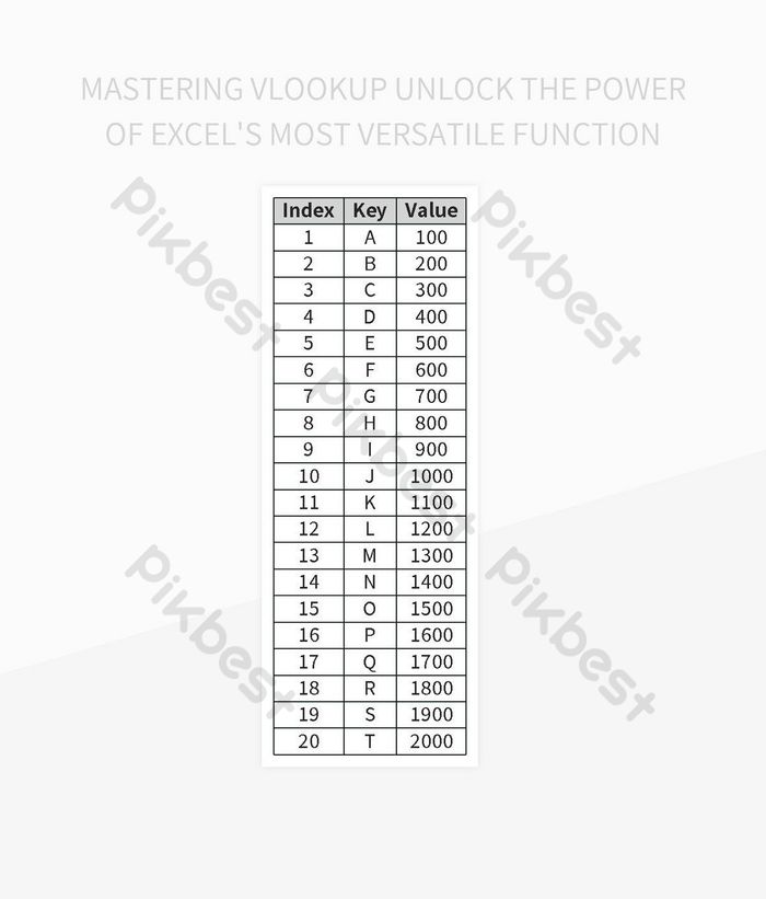
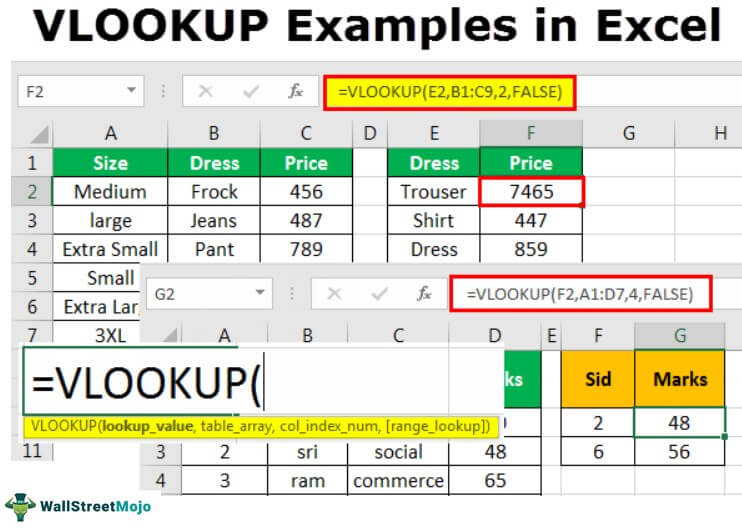
VLOOKUP stands for Vertical Lookup. It is designed to search for a value in the first column of a table, then return a value from the same row in another column you specify. The function looks vertically down the first column for the lookup value, hence the 'V' in VLOOKUP. Here's how you can initiate VLOOKUP:
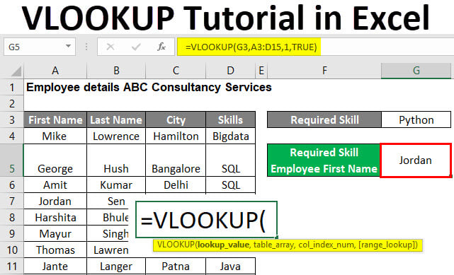
VLOOKUP(lookup_value, table_array, col_index_num, [range_lookup])
Understanding VLOOKUP Parameters

Let's break down what each of these parameters mean:
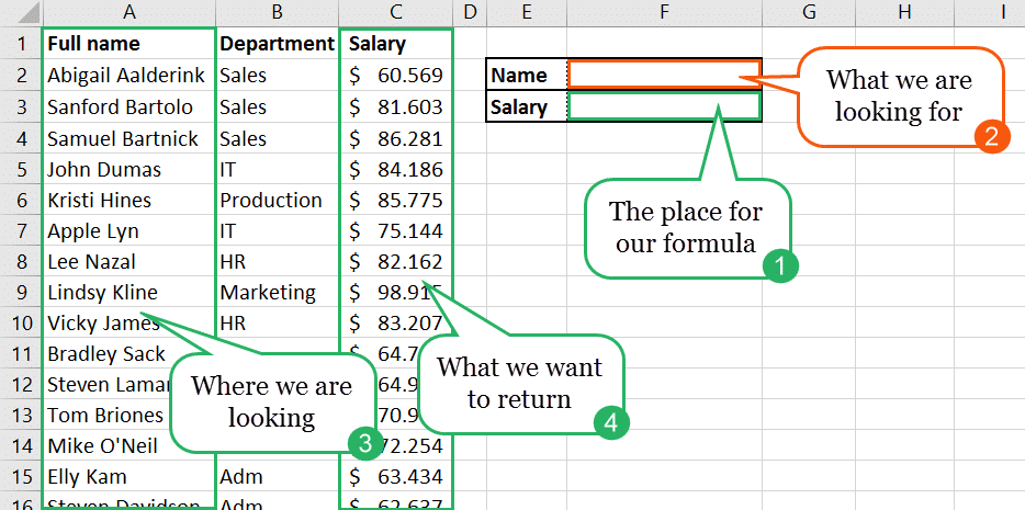
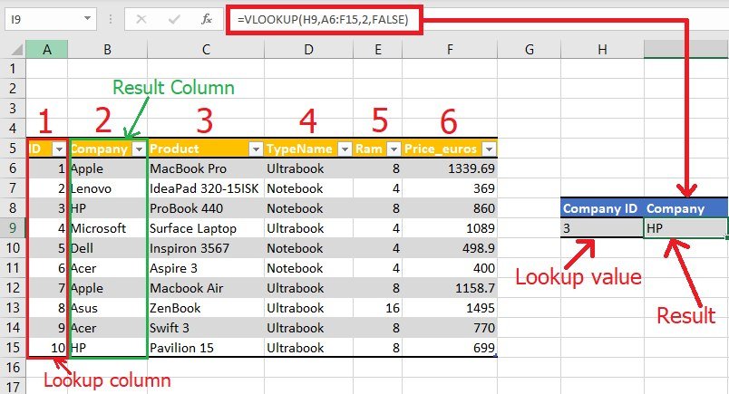
- lookup_value: The value you're searching for, which must be in the first column of your table.
- table_array: The range of cells that contains the data. This includes the lookup column and any columns you want to return data from.
- col_index_num: The column number in the table from which to retrieve the value.
- range_lookup: Optional. Enter FALSE for an exact match or TRUE for an approximate match. If omitted, TRUE is assumed.
How to Use VLOOKUP

To illustrate, let's use a basic example:
Assume you have a spreadsheet with employee data, structured like this:
| Employee ID | Name | Department | Salary |
|---|---|---|---|
| 1 | John Doe | HR | $50,000 |
| 2 | Jane Smith | Finance | $60,000 |
| 3 | Mike Brown | IT | $75,000 |

Here's how you would use VLOOKUP to find Jane Smith's salary:
- Identify the lookup value: In this case, Jane's employee ID (which is 2).
- Define the table array: This includes cells A1:D4 (assuming headers are in row 1).
- Determine the column index number: Jane's salary is in the fourth column, so the index number is 4.
- Set the range lookup: If you need an exact match, use FALSE.
The formula would look like this:
=VLOOKUP(2, A1:D4, 4, FALSE)
This function searches for the ID "2" in the first column, matches it, and returns the corresponding value from the fourth column, which is Jane's salary.
VLOOKUP Tips and Tricks
Here are some practical tips to enhance your VLOOKUP usage:
- Sort Your Data: For approximate matches, your data should be sorted in ascending order by the lookup column.
- Handle Errors: Use the
IFERRORfunction to handle VLOOKUP errors gracefully, like=IFERROR(VLOOKUP(lookup_value, table_array, col_index_num, FALSE), "Value not found"). - Expand Column References: When your table array extends over many columns, consider using a named range or a table to make your formulas easier to read and manage.
- Combining VLOOKUP with Other Functions: You can nest VLOOKUP with functions like
CHOOSEorIFfor more complex lookups.
🔍 Note: VLOOKUP is less flexible than some alternatives like INDEX and MATCH, but it's widely used due to its simplicity and straightforwardness.
⚠️ Note: Be cautious with column indexes; if you insert or delete columns, your VLOOKUP formula might break.
Common Pitfalls to Avoid
Here are some common issues you might encounter with VLOOKUP:
- Incorrect Range Lookup: Omitting the FALSE parameter can lead to unexpected results when an exact match is needed.
- Data Mismatch: VLOOKUP is sensitive to data types, so ensure your lookup value exactly matches the data in your table.
- Column Drift: If you add or remove columns in your table, your VLOOKUP might return data from the wrong column.
VLOOKUP Alternatives

While VLOOKUP is popular, there are alternatives worth exploring:
- INDEX and MATCH: This combination allows you to look up both rows and columns, offering more flexibility than VLOOKUP alone.
- XLOOKUP: Available in newer versions of Excel, XLOOKUP replaces VLOOKUP with enhanced functionality.
🌟 Note: If possible, consider using XLOOKUP for its superior capabilities and ease of use.
Wrapping up this guide on VLOOKUP, we've explored its core components, usage, and the common challenges you might face. By understanding how to effectively use VLOOKUP, you can streamline your data retrieval processes, making your work with spreadsheets much more efficient. Remember, while VLOOKUP is an essential tool, don't overlook alternatives that might serve you better in specific scenarios. Whether you're managing large datasets or performing simple lookups, Excel's VLOOKUP function can be a valuable addition to your toolkit.
Can VLOOKUP look up to the left?
+
No, VLOOKUP can only look to the right from the lookup column. If you need to look to the left, consider using INDEX and MATCH or XLOOKUP.
What happens if VLOOKUP doesn’t find a match?

+
By default, VLOOKUP will return #N/A if it doesn’t find a match. You can use IFERROR to handle this error gracefully.
How can I make my VLOOKUP more dynamic?
+
Use Excel tables or named ranges. Dynamic ranges allow your VLOOKUP formula to adjust automatically as your data changes.


