5 Simple Ways to Link Excel Sheets for Better Productivity

In today's fast-paced work environment, productivity tools like Microsoft Excel have become indispensable for managing data, tracking progress, and simplifying workflows. One of the many features that can significantly boost your productivity is linking Excel sheets. When done correctly, linking sheets allows for real-time data updates, streamlined workflows, and reduced errors, thus enhancing productivity. Here are five simple ways to link Excel sheets to help you work smarter and faster:
1. Using External References (Formulas)

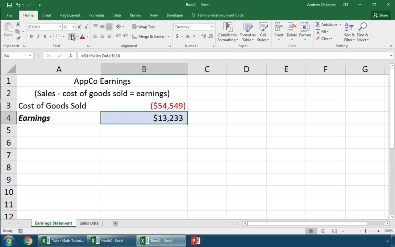
One of the most straightforward methods to link sheets is through the use of external references. Here’s how you can do it:
- Select the cell where you want to display the linked data.
- Enter
=, navigate to the other sheet (by clicking the corresponding tab or entering its name), and select the cell you want to reference. - If your sheet is named “Sheet1” and you’re linking from “Sheet2”, you’d type something like
=Sheet1!A1.
💡 Note: This method is excellent for static data or when you're linking to a single cell or a range of cells.
2. Hyperlinks

Hyperlinks can link to different sheets or even to external documents or web pages:
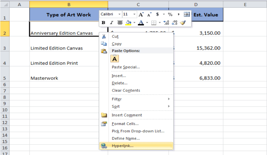
- Right-click on the cell where you want the hyperlink.
- Choose “Link” or “Insert Hyperlink.”
- Select “Place in This Document” for Excel sheets, and choose the destination sheet or cell.
3. Data Consolidation

For scenarios where you have similar data spread across multiple sheets, data consolidation can be your go-to:
- Go to “Data” > “Consolidate” in Excel’s ribbon.
- Choose the function you want to apply (Sum, Average, etc.).
- Select the ranges from each sheet you want to consolidate.
| Sheet Name | Data Range | Function |
|---|---|---|
| Sheet1 | A1:A10 | Sum |
| Sheet2 | A1:A10 | Sum |

💡 Note: If the sheets have different structures or layouts, you might need to adjust or align them manually before consolidating.
4. Using VLOOKUP or Index-Match

When you need to pull data from one sheet based on a lookup value, VLOOKUP or the more flexible Index-Match can be used:
- For VLOOKUP:
- Enter
=VLOOKUP(lookup_value, table_array, col_index_num, [range_lookup])with the table_array referencing another sheet. - Example:
=VLOOKUP(A2, Sheet1!A1:B10, 2, FALSE).
- Enter
- For Index-Match:
- Use
=INDEX(return_range, MATCH(lookup_value, lookup_range, 0)). - Example:
=INDEX(Sheet1!B:B, MATCH(A2, Sheet1!A:A, 0)).
- Use
5. Creating Dynamic Named Ranges

Named ranges can make referencing easier and more dynamic:
- Define a named range using “Formulas” > “Define Name.”
- Use OFFSET or INDEX to create a dynamic range. Here’s a simple OFFSET example:
=OFFSET(Sheet1!A1,0,0,COUNTA(Sheet1!A:A),1)
- Now, use this named range in formulas across different sheets.
By linking your Excel sheets using these methods, you not only streamline your data management but also ensure that your spreadsheets remain accurate and up-to-date. Remember, the key to productivity with Excel is not just knowing what tools are available, but understanding how to use them effectively to meet your unique needs.
Can I link Excel sheets from different files?

+
Yes, you can link Excel sheets from different files by using external references, ensuring the file paths are correctly referenced in your formulas.
What happens when a linked sheet changes?

+
Any changes made to the source sheet will automatically update in all cells or sheets that reference it, as long as they are within the same workbook. However, you might need to refresh links for changes in external files.
How do I prevent circular references when linking sheets?

+
Avoid circular references by ensuring that a cell does not directly or indirectly refer to itself. Use formulas and external references carefully, and ensure there’s a clear flow from input to output cells.