Compare Excel Columns Easily with VLOOKUP Guide

In today's data-driven world, efficiently comparing datasets is essential for insightful analysis and decision-making. Microsoft Excel offers a plethora of functions to handle such tasks, and VLOOKUP stands out as a versatile tool for this purpose. Whether you're reconciling financial records, validating databases, or simply comparing lists, mastering the VLOOKUP function can significantly streamline your workflow. This comprehensive guide will delve into how to use VLOOKUP to compare columns, offering step-by-step instructions, practical examples, and expert tips.
Understanding VLOOKUP

VLOOKUP, or Vertical Lookup, is designed to search for a value in the first column of a table and return a value in the same row from another specified column. Here’s the syntax:
- lookup_value: The value you want to search for.
- table_array: The range containing the lookup value and the result you want to return.
- col_index_num: The column number in the table from which to retrieve the value.
- [range_lookup]: Optional argument specifying whether you need an exact match (FALSE) or approximate match (TRUE).

VLOOKUP is particularly useful when comparing two lists:
- To find missing entries in one list.
- To identify differences between values.
- To merge data from different tables based on a common identifier.
Comparing Excel Columns with VLOOKUP

Step-by-Step Guide

1. Setting Up Your Data:
- Ensure your datasets are in separate columns. For example, place one list in columns A and B, and the other in columns D and E.
- Make sure there's a common identifier that can be used for comparison.
2. Basic VLOOKUP Syntax:
Let's say you want to compare values in column A with values in column D:
=VLOOKUP(A2, $D$2:$E$10, 1, FALSE)
- Here, A2 is the lookup_value (value to search).
- $D$2:$E$10 is the table_array (the range of columns D and E where the lookup will happen).
- The number 1 indicates we're looking in the first column of the table_array for the lookup_value.
- FALSE ensures an exact match is required.
3. Comparing Lists:
- In a new column, enter the above formula. Drag the formula down to compare all values.
- If the formula returns #N/A, it means the value is not found in the second list.
Example of Column Comparison

| Column A (Lookup Values) | Column B (Details) | Column D (Compare Values) | Column E (Details) | Column F (Result) |
|---|---|---|---|---|
| Apple | Fruit | Apple | Fruit | Apple |
| Banana | Fruit | Cherry | Fruit | #N/A |
| Cherry | Fruit | Banana | Fruit | Banana |

In this example, you can see that "Apple" is found in both lists, but "Banana" in column A is not found in the second list, and "Cherry" in column D does not appear in column A.
4. Highlighting Differences:
To highlight differences visually:
- Use Conditional Formatting with a formula like:
- This formula will return TRUE where the lookup value from column A does not exist in column D, allowing you to apply color formatting to those cells.
=ISNA(VLOOKUP(A2, $D$2:$D$10, 1, FALSE))
5. Avoiding Common Errors:
- Ensure the lookup column is the leftmost column in the table_array.
- Check for any leading or trailing spaces in your data that might cause false negatives.
- Always use absolute references for the table_array to prevent formula errors when copying down.
🔍 Note: Remember to align your data correctly in Excel. If your lookup values are not in the first column of the table_array, VLOOKUP will not work correctly.
Advanced Tips and Techniques

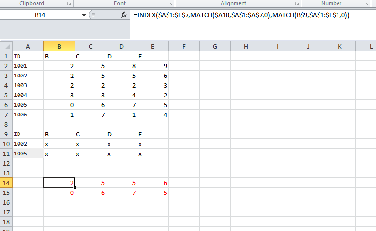
- Using INDEX and MATCH: While VLOOKUP is powerful, combining INDEX and MATCH can offer more flexibility, especially for larger datasets.
- Handling Errors: Use IFERROR with VLOOKUP to display alternative messages or values instead of the standard error messages.
- Sorting Data: If using approximate match (TRUE), your data needs to be sorted in ascending order based on the lookup column.
By mastering these techniques, you can not only compare columns with ease but also enhance your Excel proficiency, making you invaluable in data management and analysis roles.
Wrapping Up

Throughout this guide, we explored the powerful capabilities of the VLOOKUP function in Excel for column comparison. From setting up your data correctly, understanding the syntax, to practical examples and advanced techniques, VLOOKUP is indeed an indispensable tool in your Excel toolkit. Whether you’re cross-referencing data, verifying entries, or preparing for data analysis, mastering VLOOKUP can significantly enhance your productivity and accuracy in data handling. Remember, the key to mastering this function lies in practice and understanding how to tweak its parameters to fit your specific needs.
Why does VLOOKUP return #N/A?

+
VLOOKUP returns #N/A when the lookup_value is not found in the first column of the table_array. This could be due to data entry errors, misaligned ranges, or if the exact match parameter (FALSE) is set when an approximate match should be used.
Can VLOOKUP look to the left?

+
No, VLOOKUP cannot natively look to the left; it always looks for the lookup_value in the first column of the table_array. However, you can use INDEX and MATCH functions together to achieve similar results with more flexibility.
How can I make VLOOKUP case-sensitive?

+
VLOOKUP by itself is not case-sensitive. However, you can use a helper column with EXACT or FIND functions to make a comparison case-sensitive and then VLOOKUP or combine with IF or CHOOSE functions to achieve case sensitivity.