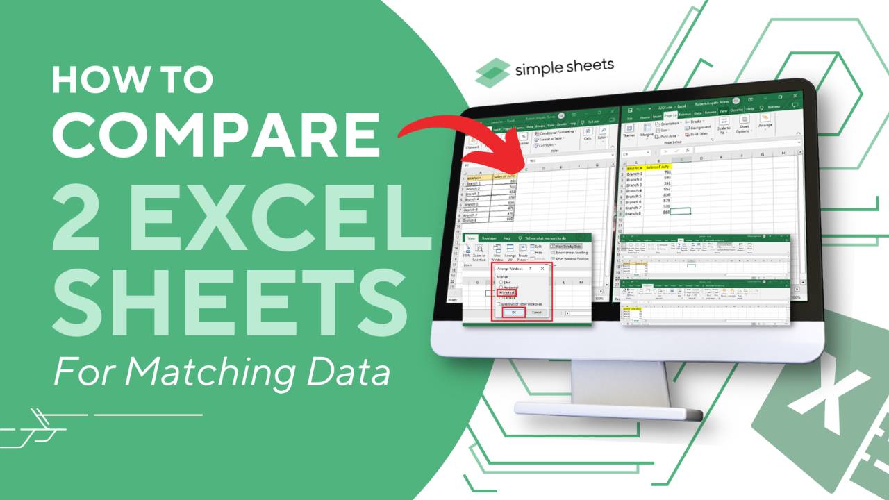
3 Ways to Compare Excel Columns Across Sheets

When dealing with multiple datasets in Microsoft Excel, one common task is to compare columns across different sheets. Whether you're syncing data, identifying differences, or merging information, understanding how to effectively compare columns can save time and reduce errors. Here are three practical methods to achieve this:

Method 1: Using VLOOKUP for Simple Matching

VLOOKUP (Vertical Lookup) is a straightforward Excel function often used to find and retrieve data in a column. Here’s how you can use it to compare columns:

• Identify the Column to Look Up: Choose the column you want to compare. Let's say this is Column A in Sheet1.
• Set Up the VLOOKUP Formula: In Sheet2, next to the column you want to match, write:

  =VLOOKUP(A1,Sheet1!A:A,1,FALSE)

Where:
• A1 is the first cell to compare in Sheet2.
• Sheet1!A:A is the entire column A from Sheet1 to search in.
• 1 indicates we want the value from the first column.
• FALSE ensures an exact match.
• Drag the Formula Down: Drag this formula down to fill the entire column where you want to match data.

👀 Note: If there's no match, VLOOKUP will return #N/A. Use IFERROR to handle these errors if you prefer, like =IFERROR(VLOOKUP(A1,Sheet1!A:A,1,FALSE),"Not Found").

Method 2: Conditional Formatting for Visual Comparison

For a quick visual comparison, Conditional Formatting is highly effective:

• Select the Range: Choose the range of cells in Sheet2 that you want to compare.
• Open Conditional Formatting:

  Home > Conditional Formatting > New Rule > Use a formula to determine which cells to format

• Create the Rule: Use the following formula:

  =A1<>Sheet1!A1

Where A1 is the first cell you're comparing, adjusting as needed.
• Select a Formatting Option: Choose how differences should be highlighted, such as with a fill color.
• Apply Rule: Click OK to apply the rule. Any cells that differ will be visually highlighted.

💡 Note: You can use this method to compare entire columns or only specific ranges, making it versatile for various comparison needs.

Method 3: Using Power Query for Advanced Data Comparison

Power Query in Excel provides robust tools for data manipulation and comparison:

• Open Power Query:

  Data > Get & Transform Data > Get Data > From Other Sources > Blank Query

• Load Data:
• Click on "Advanced Editor" and write M code to load data from both sheets:

    let
        Source = Excel.CurrentWorkbook(){[Name="Sheet1"]}[Content],
        Sheet2 = Excel.CurrentWorkbook(){[Name="Sheet2"]}[Content]
    in
        {"Sheet1", Source},
        {"Sheet2", Sheet2}

• Combine and Compare: Use Power Query's Merge function to align and compare data:

    Merge = Table.NestedJoin(Source, {"Column1"}, Sheet2, {"Column1"}, "NewSheet")

• Expand and Filter: Expand the merged table and filter to show only differences or matches based on your criteria.
• Load the Query: Once satisfied with the comparison, load the results back into Excel.

This method is particularly useful for large datasets where simple VLOOKUP or conditional formatting might be inefficient.

📝 Note: Power Query requires a basic understanding of its query language and functions but offers unmatched flexibility for complex data operations.

The methods described above cater to different needs, from simple value matching to complex data analysis. Choosing the right method depends on your dataset size, the level of detail you need, and your familiarity with Excel's tools. VLOOKUP provides immediate results for straightforward comparisons, Conditional Formatting gives a quick visual cue for mismatches, and Power Query allows for in-depth analysis and transformation of data. Each approach has its place in your Excel toolkit, enhancing your ability to manage, compare, and analyze data efficiently.

What is the main advantage of using VLOOKUP for column comparison?

+

VLOOKUP is straightforward and quickly identifies if a value exists in another sheet, making it ideal for simple matching tasks.

How can Conditional Formatting be used for comparing data visually?

+

By applying rules that highlight cells where values differ between two columns, Conditional Formatting visually aids in spotting discrepancies or unique entries.

When should I use Power Query for data comparison?

+

Use Power Query for complex comparisons involving large datasets or when you need to transform data before comparing. Its ability to merge, clean, and transform data makes it suitable for advanced analysis.