Effortlessly Compare Columns in Excel: A Quick Guide

If you find yourself dealing with extensive data sets in Microsoft Excel, the ability to compare columns effectively can make your work significantly more manageable. Excel offers various tools and techniques for comparing columns, helping users to identify discrepancies, find matches, or determine differences within seconds. Whether you're a financial analyst reconciling accounts, a marketer analyzing customer data, or just managing your personal budget, mastering column comparison in Excel can be a game-changer.
Why Compare Columns in Excel?

Before we delve into the mechanics of how to compare columns in Excel, understanding why you might need to do this can contextualize the process:
- Data Validation: Ensuring that your data entries across different spreadsheets or sections are consistent.
- Spotting Anomalies: Quickly identifying outliers or errors in large datasets.
- Duplicate Detection: Finding and managing duplicate entries or records.
- Change Tracking: Monitoring changes or updates in different versions of datasets.
- Efficiency: Streamlining workflows by reducing manual comparison and verification time.
Methods to Compare Columns in Excel

Here are some of the most effective methods to compare columns in Excel:
1. Using Conditional Formatting

Conditional formatting is one of the simplest yet powerful tools for visual comparison:
- Select the two columns you want to compare.
- Go to the Home tab, click on Conditional Formatting, then select New Rule.
- Choose Use a formula to determine which cells to format.
- Enter this formula to highlight cells in the first column where values differ from the second column:
=A2<>B2(replace A2 and B2 with your column references). - Set the format style you want to apply when the condition is true (e.g., a different cell color).
This method instantly shows where differences exist by changing the appearance of cells, making it easy to spot discrepancies at a glance.
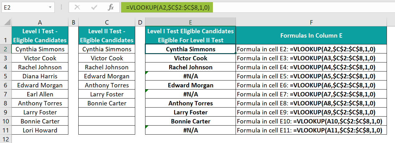
2. Utilizing VLOOKUP for Exact Matches

The VLOOKUP function allows you to compare data between columns by searching for a value in one column and returning a corresponding value from another column:
- In a new column (say, C), enter
=IFERROR(VLOOKUP(A2,B2:B100,1,FALSE),“Not Found”). - Press Enter to apply the formula.
- Drag the formula down to apply it to all cells in column A.
This will return “Not Found” if the value in column A is not present in column B.
3. The COUNTIF Function for Finding Duplicates

To identify duplicates between two columns:
- Select an empty column © next to the columns you’re comparing.
- Type in
=IF(COUNTIF(B:B,A2)>=1, “Duplicate”, “Unique”). - Hit Enter and drag the fill handle down to fill the formula for the entire range.
Excel will label each value as “Duplicate” or “Unique” based on its presence in the other column.
| Column A | Column B | Comparison Result |
|---|---|---|
| Apple | Banana | Unique |
| Apple | Apple | Duplicate |

4. Using Power Query for Advanced Comparison

For more complex datasets, Power Query in Excel can be very effective:
- Load your data into Power Query by selecting your range and choosing From Table/Range.
- Use the Merge Queries option to join your two tables or columns.
- Set the join key to the column you wish to compare.
- Select the operation type like Inner Join or Full Outer Join to identify matches or non-matches.
- Return the query to Excel for analysis.
5. VBA for Customized Comparison

For users comfortable with VBA, writing a macro can automate and customize column comparisons:
Sub CompareColumns() Dim ws As Worksheet Dim lastRowA As Long, lastRowB As Long Dim cell As Range Set ws = ThisWorkbook.Sheets(“Sheet1”) ‘replace with your sheet namelastRowA = ws.Cells(ws.Rows.Count, "A").End(xlUp).Row lastRowB = ws.Cells(ws.Rows.Count, "B").End(xlUp).Row For Each cell In ws.Range("A1:A" & lastRowA) If cell.Value <> ws.Cells(cell.Row, "B").Value Then cell.Offset(0, 2).Value = "Differs" Else cell.Offset(0, 2).Value = "Same" End If Next cell
End Sub
This VBA script compares values in columns A and B and places results in column C.
💡 Note: Always make a backup before running macros on your data to prevent unintended changes.
Throughout this post, we've explored various methods to compare columns in Excel, catering to different needs from simple visual differentiation to complex data reconciliation. Each method has its place depending on your specific requirements, the size of your dataset, and your comfort level with Excel's functions and tools. By leveraging these techniques, you can significantly reduce the time and effort required for data analysis, enhancing both productivity and accuracy in your work.
Can I compare more than two columns at once?

+
Yes, you can extend the Conditional Formatting or VBA methods to compare multiple columns, though it might become complex. Power Query is particularly effective for comparing multiple columns with different datasets.
How can I highlight only unique values?

+
Use the Conditional Formatting rule with the formula like =COUNTIF(B:B,A2)=0 to highlight unique values in Column A.
What should I do if my data contains blanks?

+
Blanks can affect comparison results. You might want to filter out blanks or handle them specifically in your formula or script. For example, modify the formula to ignore blanks: =IF(A2=“”,“”,A2<>B2)