Comparing Two Excel Columns: Simplified Guide

Understanding the Basics

Comparing two Excel columns is a common task in data analysis that can save you hours of manual checking. Whether you need to find matches, differences, or duplicates, Excel offers multiple ways to make this task quick and efficient. In this guide, we’ll explore various methods to compare two columns in Excel, from simple conditional formatting to more advanced formulas.
Why Compare Columns?

Before delving into the how-to, let’s understand why comparing columns is essential:
- Data Validation: Ensuring data integrity by checking for consistency.
- Duplicate Detection: Identifying repetitive entries in datasets.
- Mismatch Analysis: Finding discrepancies between two data sets, perhaps from different sources or periods.
Method 1: Conditional Formatting

One of the simplest ways to visually compare two columns is by using conditional formatting. Here’s how:
- Select the range of cells you want to compare, ensuring both columns are included.
- Go to Home > Conditional Formatting > New Rule…
- Choose “Use a formula to determine which cells to format.”
- Enter the formula:
=A1=B1if comparing cells in column A and B, or=NOT(A1=B1)to highlight differences. - Set the format to change the cell’s color if the condition is met.
💡 Note: Conditional formatting can only show the differences or matches visually but won't automatically tell you the count or type of matches.
Method 2: Using Formulas

Excel formulas offer a more dynamic way to compare data:
- VLOOKUP:
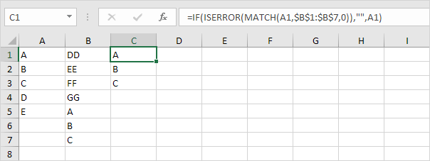
If the result matches A1, it means there’s a match; if it returns #N/A, there isn’t.=VLOOKUP(A1, B1:B10, 1, FALSE)
<li><strong>IF & EXACT:</strong>
=IF(EXACT(A1, B1), "Match", "No Match")
📝 Note: Use IF and EXACT for exact matches to prevent case-sensitive mismatches.
Method 3: Using Vlookup with Helper Column

If you want to count or identify the total number of matches:
- Create a helper column (e.g., column C) next to the columns you are comparing.
- Use VLOOKUP to find matches or mismatches in this new column:
=IFERROR(VLOOKUP(A1, $B$1:$B$10, 1, FALSE), "Mismatch") - Then, you can count matches or mismatches with COUNTIF or SUMIF:
or=COUNTIF(C1:C10, "Match")=COUNTIF(C1:C10, "Mismatch")
Method 4: Using a Table

Another efficient way to compare two columns is through Excel tables. Here's how to set it up:
| Column A | Column B | Result |
|---|---|---|
| 123 | 123 | Match |
| abc | def | Differ |

Below is the formula you would use in the "Result" column:
=IF(A2=B2, "Match", "Differ")
Wrapping Up

Comparing two columns in Excel isn’t just about finding differences; it’s about understanding your data better. By using conditional formatting, formulas, or structured tables, you can quickly highlight, count, or analyze matches and discrepancies. Each method has its place, depending on your needs for presentation, automation, or data analysis. From simple to advanced techniques, Excel provides robust tools for data comparison that can streamline your workflow, ensuring accuracy and efficiency in your data management tasks.
What is the best method to visually compare two columns?

+
For visual comparison, conditional formatting offers an immediate and intuitive way to see matches and differences by color coding the cells.
Can Excel handle case sensitivity while comparing columns?

+
Yes, by using functions like EXACT or by configuring the comparison formula to be case-sensitive, Excel can differentiate between ‘Apple’ and ‘apple’.
How do I find duplicates in two columns?

+
Create a helper column using VLOOKUP or COUNTIF to identify duplicates or use conditional formatting to highlight cells that appear more than once in both columns.