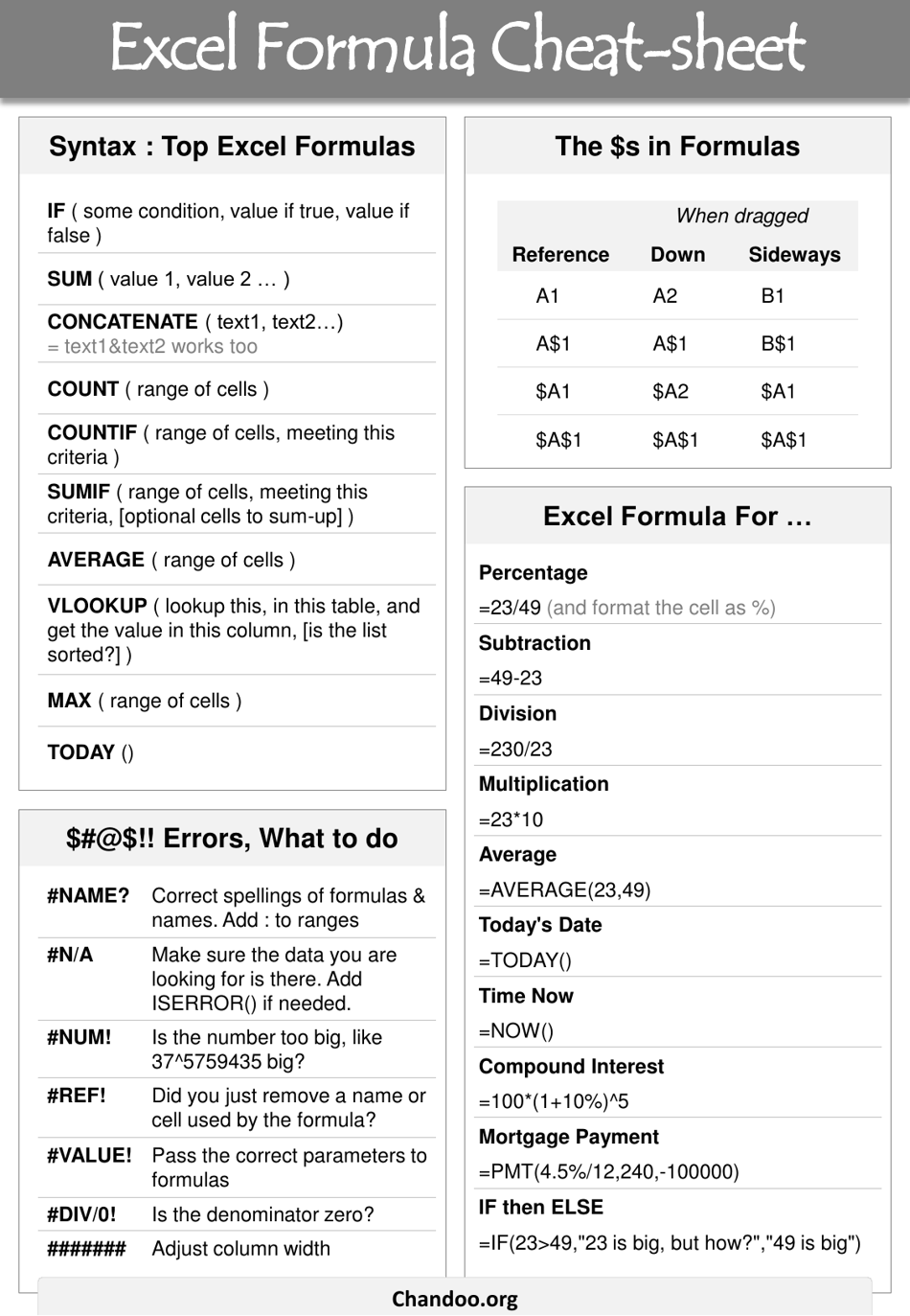
Excel Magic: 5 Simple Tips for Formulas

Mastering Excel formulas can transform your experience with Microsoft Excel from a mere data-entry tool to a powerful engine for calculations and data analysis. Whether you're new to Excel or looking to refresh your knowledge, understanding the simplicity yet depth of Excel formulas is crucial. Here are five simple tips to help you harness the power of Excel formulas.
1. Keep It Simple with Named Ranges

Before diving deep into complex formulas, leveraging named ranges in Excel can simplify formula creation and make them easier to read and maintain. Instead of using cell references like A1 or C1:C10, you can name these ranges to reflect what they represent.
- To create a named range, select the cell or range you want to name, go to the ‘Formulas’ tab, and click on ‘Define Name’. Here you can enter a name like ‘Sales’ for your sales data.
- When you need to use this data in a formula, instead of typing
=SUM(A1:A10), you can simply write=SUM(Sales). This makes formulas much more intuitive.
💡 Note: Ensure that your named ranges are distinct to avoid conflicts with other range names or cell addresses.
2. Utilize Logical Functions for Conditional Operations

Logical functions like IF, AND, OR, NOT can handle complex conditional statements in your data analysis.
- IF function allows you to perform calculations based on whether a certain condition is true or false.
- You can use AND/OR within an IF statement to test multiple conditions.
- Nested IF statements can extend this capability, but remember, too many nested IFs can make your formula unwieldy.
Here’s an example:
=IF(B2>1000,“Bonus: 200",IF(AND(B2>500,B2<=1000),"Bonus: 100”,“No Bonus”))
3. Master the Power of Array Formulas

Array formulas in Excel enable you to perform multiple calculations on one or more items in an array with a single formula. They’re incredibly powerful for:
- Complex calculations involving multiple cells or ranges.
- Processing data in a way that regular formulas can’t.
Here is an example of an array formula to sum the product of two columns:
=SUM(B2:B10*C2:C10)
To enter an array formula, you would typically type it and then press Ctrl+Shift+Enter (for older Excel versions). Modern Excel versions now recognize array formulas automatically.
📝 Note: Remember to double-check your array formula results, especially with older Excel versions where you might need to enter them as CSE (Control Shift Enter) formulas.
4. Utilize Lookup Functions for Data Retrieval

The VLOOKUP and HLOOKUP functions, along with their newer siblings XLOOKUP and INDEX/MATCH, are essential for retrieving data from tables:
- VLOOKUP looks up values vertically, which is perfect for tables where data is organized in columns.
- HLOOKUP searches horizontally in the first row of a table.
- XLOOKUP provides more flexibility and replaces both VLOOKUP and HLOOKUP with more robust functionality.
- INDEX/MATCH gives you dynamic lookup capabilities where VLOOKUP might fall short.
An example of VLOOKUP:
=VLOOKUP(D2, A1:C10, 3, FALSE)
This formula looks up the value in D2 within the first column of A1:C10 and returns the value from the third column of that range if an exact match is found.
5. Use Error Handling to Make Formulas Robust

In real-world scenarios, data is not always clean, and this can lead to errors in formulas. Here’s how to make your formulas more resilient:
- Use the IFERROR function to handle potential errors gracefully. It allows you to specify what should be displayed if an error occurs.
- For instance,
=IFERROR(VLOOKUP(E2, A1:C10, 3, FALSE), "Not Found")will display “Not Found” if the VLOOKUP does not find a match or if there’s any error.
✅ Note: When using error handling, consider the types of errors that might occur and tailor your responses to each specific scenario.
In conclusion, Excel formulas can significantly enhance your productivity and data analysis capabilities. From simplifying your spreadsheets with named ranges to handling complex data with logical and array formulas, mastering these tips will help you navigate Excel with greater ease and accuracy. By combining these techniques, you can create robust, dynamic, and efficient spreadsheets that cater to your analytical needs. Whether you're managing business data, personal finance, or any other kind of information, Excel's formula power is at your fingertips to unlock insights and drive decision-making.
What is a named range in Excel?

+
A named range in Excel is a user-defined name assigned to a specific cell or range of cells, allowing for easier reference in formulas and making spreadsheets more intuitive and less prone to errors due to cell reference changes.
How can I use VLOOKUP in Excel?

+
To use VLOOKUP, you need to specify the lookup value, the table array (where the data is stored), the column index number from which to retrieve the value, and optionally, the range lookup argument to decide if you want an exact or approximate match.
What are the advantages of using array formulas?

+
Array formulas offer several advantages, including performing complex calculations in a single formula, dealing with arrays of data without the need for multiple intermediate steps, and processing multiple values or criteria simultaneously.