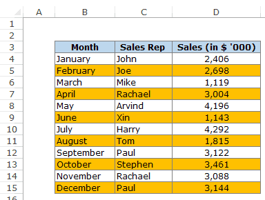
5 Ways to Alternate Row Colors in Excel 2007

Mastering the art of data visualization in Excel can significantly enhance your ability to interpret and present data effectively. One of the simplest yet most impactful ways to improve the readability of your spreadsheets is by using alternating row colors or what is commonly known as "zebra stripes." This article will guide you through five different methods to achieve this in Excel 2007, ensuring your data stands out with clarity and style.

Method 1: Using Conditional Formatting

Conditional Formatting in Excel 2007 allows you to apply different styles to rows based on their position, making it easy to implement alternating row colors.

1. Select the range of cells you want to format.
2. Go to the Home tab and click on “Conditional Formatting” in the Styles group.
3. Choose “New Rule” from the dropdown.
4. In the New Formatting Rule dialog, select “Use a formula to determine which cells to format.”
5. Enter the formula: =MOD(ROW(),2)=0 for even rows or =MOD(ROW(),2)=1 for odd rows.
6. Click on “Format” to open the Format Cells dialog, select your preferred color under the Fill tab, and then click OK.
7. Back in the New Formatting Rule dialog, click OK to apply the formatting.

🔎 Note: This method dynamically formats rows, which means if you add or remove rows, the formatting will adjust automatically.

Method 2: Table Format

If you use tables in Excel, you can easily apply alternating row colors without any complex formulas or manual formatting.

1. Select your data range.
2. From the Home tab, click on “Format as Table.”
3. Choose one of the table styles that feature alternating row colors. Excel 2007 offers multiple styles to choose from, ensuring you can find one that matches your report’s aesthetics.

🔍 Note: This method makes your data instantly recognizable as a table, which also provides additional functionalities like sorting and filtering.

Method 3: Manual Selection

For small datasets or if you need a one-time setup, you might prefer to manually highlight rows.

1. Select the rows you wish to color.
2. Use the Fill Color button in the Home tab to apply a background color.
3. Repeat for alternate rows using a different color or leaving them blank for contrast.

Method 4: VBA Macro

For users who frequently need to apply alternating row colors or work with large datasets, a VBA macro can automate this task.

1. Press ALT + F11 to open the VBA editor.
2. Insert a new module (Insert > Module).
3. Enter the following VBA code:

Sub AlternateRowColor()
    Dim rng As Range
    Set rng = Selection
    For i = 2 To rng.Rows.Count Step 2
        rng.Rows(i).Interior.Color = RGB(220, 220, 220)
    Next i
End Sub

4. Close the VBA editor and return to Excel.
5. To run the macro, select your data range, press ALT + F8, select “AlternateRowColor” and click “Run.”

🎯 Note: This macro uses a gray background color for even rows, but you can adjust the RGB values to match your desired color scheme.

Method 5: Using Named Ranges and Formulas

This method uses named ranges and the ROW function to apply colors conditionally.

1. Define a named range for your data set. For example, call it “MyData.”
2. Go to Conditional Formatting and choose “New Rule” as before.
3. Use the formula: =MOD(ROW()-ROW(MyData)+1,2)=0 for even rows or =MOD(ROW()-ROW(MyData)+1,2)=1 for odd rows.
4. Set the desired format and apply it.

🔎 Note: This method is particularly useful if you want to apply different formatting rules based on the range’s position relative to a fixed point.

As you've seen, there are multiple ways to alternate row colors in Excel 2007, each with its advantages depending on your needs. Whether you're looking for a dynamic solution that adapts as you modify your data, or prefer a one-time manual setup, Excel offers versatile options to enhance the visual appeal of your spreadsheets. Choosing the right method can streamline your work, ensuring that your data is not only functional but also visually pleasing. Remember to consider your data's size, how often it changes, and the level of control you want over the presentation when deciding which technique to use.

Can I change the color pattern after applying a method?

+

Yes, you can modify the color settings in any method by either changing the formatting rule, editing the table style, or altering the VBA macro code.

Will these methods work on filtered data?

+

Conditional Formatting and Table Formatting will adapt to filtered data by only applying the colors to visible rows. VBA and manual methods might require you to adjust the selection or code to account for filtering.

Is there a way to remove alternate row colors?

+

To remove these colors, you would undo the respective formatting or macro execution. For Conditional Formatting, select the cells and clear the rules. For tables, choose a ‘none’ style or remove table formatting.

Can I apply these methods to an entire worksheet?

+

Yes, you can select the entire worksheet (by clicking the corner button above the row numbers and to the left of the column letters) before applying any of these methods, though remember that the “Table Format” method might not be suitable for the entire sheet.