5 Ways to Reference Another Sheet in Excel Easily

In today's dynamic data environment, the ability to connect and manipulate data from different Excel sheets becomes essential. This post outlines five straightforward methods to reference data from another sheet within Excel, enhancing your efficiency in data management:
Method 1: Direct Cell Reference

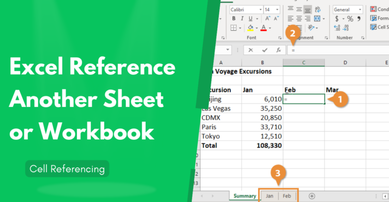
One of the most straightforward ways to reference data from another sheet is through direct cell referencing. Here’s how:
- Open the workbook where you need to make references.
- Go to the cell where you want to pull in data.
- Type the equal sign (=) followed by the sheet name, an exclamation mark (!), and the cell reference. For example, to reference cell A1 from Sheet2 in Sheet1, you would type:
=Sheet2!A1. - If your sheet name contains spaces or special characters, use single quotes around the sheet name, like this:
=‘Sheet Two’!A1.
💡 Note: Always ensure that sheet names do not include special characters like [ ] or ? when not using quotes, as these can interfere with the formula.
Method 2: Using Named Ranges

Named ranges can make your formulas much more readable and easier to manage:
- Select the range you want to name in the source sheet.
- Go to the “Formulas” tab, choose “Define Name,” and give your range a meaningful name.
- In the cell of your destination sheet, you can then reference this named range. For example, if you’ve named a range ‘SalesData’, you can reference it by typing:
=SalesData.
Using named ranges simplifies formula maintenance and aids in debugging complex spreadsheets.
Method 3: VLOOKUP or INDEX/MATCH

If you’re looking to reference data based on matching criteria:
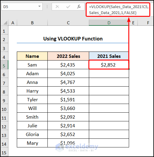
- VLOOKUP: Use this to find and retrieve data based on a lookup value. For instance, to find a product name in ‘Products’ sheet based on SKU in ‘Sales’ sheet:
=VLOOKUP(A2,Products!A:B,2,FALSE). - INDEX/MATCH: Offers more flexibility than VLOOKUP. Here’s how you might use it to reference data from another sheet:
=INDEX(Products!B:B,MATCH(A2,Products!A:A,0)).
These functions are particularly useful for dynamic data references where values might change or need updating.
Method 4: External References

To reference data from another workbook:
- Open both workbooks.
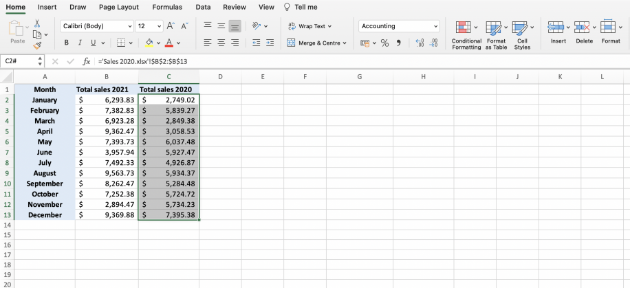
- In the cell where you want to insert the external reference, use the following formula structure:
=[Drive][Folder]Path[WorkbookName]SheetName!CellReference. For example, if your external workbook is ‘Q1Sales.xlsx’ and the sheet is ‘Sales’, you could use:=‘C:\Reports\Q1Sales.xlsx’!Sales!B2.
Method 5: 3D References

For summarizing data across multiple sheets:
- To sum values in cell A1 from ‘Sheet1’ through ‘Sheet4’, you would use:
=SUM(Sheet1:Sheet4!A1).
This method is particularly handy for aggregated reporting from multiple sheets within the same workbook.
Final Thoughts

Linking data across sheets in Excel not only increases the functionality and efficiency of your workbooks but also ensures data accuracy and consistency. Whether you’re pulling in simple cell references or compiling complex reports, understanding these methods can dramatically reduce the time you spend on data management.
Can I use these methods with Google Sheets?

+
Yes, Google Sheets supports all these methods, though some syntax and functionality might differ slightly. Named ranges, for instance, work very similarly.
What if my sheet name changes?

+
If a sheet’s name changes, all references to that sheet must be updated manually or by using the ‘Find and Replace’ feature in Excel.
Is it possible to reference cells conditionally?

+
Yes, you can use conditional formulas like IF or CHOOSE to reference cells based on specific criteria, making your spreadsheets more dynamic.