Excel Data Linking: Master Cross-Sheet Pulling

The ability to pull data from one Excel worksheet into another is not only a testament to Excel's versatility but also a crucial skill for managing complex data sets. Whether you're a financial analyst collating quarterly earnings, a project manager tracking tasks across multiple sheets, or a student compiling research data, knowing how to master cross-sheet data linking can streamline your workflow, increase accuracy, and save valuable time. Let's dive into the essentials of Excel data linking, explore some advanced techniques, and discuss common pitfalls and their solutions.
Understanding Excel Data Links

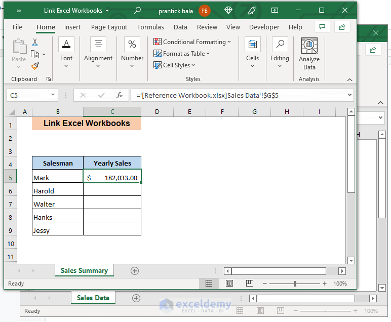
At its core, Excel data linking is about creating dynamic references to data across different sheets within the same workbook or even different workbooks. Here’s how you can get started:
- Navigate to the Cell: First, decide where you want your data to appear.
- Use the Equals Sign: Type an equals sign (=) to begin a formula.
- Select the Source Cell: Switch to the worksheet containing your data. Click the cell you want to reference.
- Return to Your Worksheet: After selecting the source, press Enter, and Excel will write a formula like
=Sheet2!A1.
Basic to Advanced Linking Techniques

Simple Cell Reference

The simplest form of linking involves directly referencing a cell from another worksheet.
=SheetName!CellAddressThis method is straightforward but not dynamic. If you insert or delete columns or rows, the reference doesn’t adjust automatically.
Using Functions for Dynamic Linking

Here are some functions that enhance the linking process:
- VLOOKUP: Use this when you want to match data from different sheets.
=VLOOKUP(lookup_value, Sheet2!A1:C10, col_index_num, FALSE) - INDEX and MATCH: A more versatile alternative to VLOOKUP, allowing for two-way lookups.
=INDEX(Sheet2!A1:A10, MATCH(value, Sheet2!B1:B10, 0)) - SUMIF or COUNTIF: Aggregate data based on conditions in another sheet.
=SUMIF(Sheet1!A1:A10, "Condition", Sheet1!B1:B10)
💡 Note: When linking with functions, ensure that your column references in VLOOKUP or row references in MATCH account for potential changes in data structure.
Named Ranges

Using named ranges can make your links more readable and less error-prone:
- Select the range of cells in the source sheet.
- Go to Formulas > Define Name and give the range a name.
- In your destination sheet, use
=NameOfRangeto pull the data.
| Action | Benefit | Example |
|---|---|---|
| Name a Range | Clarity and Ease of Use | =SalesData |
| Use in Formulas | Reduced Error Rates | =SUM(SalesData) |

Dynamic Named Ranges

To keep your data links dynamic as data grows, use OFFSET with named ranges:
=OFFSET(SalesData,0,0,COUNTA(SalesData),1)🚨 Note: Dynamic named ranges might slow down Excel with large data sets; use them judiciously.
Common Issues and Troubleshooting

Linking data across sheets can occasionally lead to errors. Here are some common problems:
- Broken Links: If the source file is moved or renamed, links break. Use absolute references or Excel’s Link Management tool to update links.
- Formula Errors: Ensure that there are no mismatches in sheet names or cell addresses. Double-check formula references.
- Volatility: Overuse of volatile functions like OFFSET or INDIRECT can slow down your workbook. Minimize their use or opt for more stable alternatives.
- Data Integrity: Incorrectly formatted cells or data types can cause unexpected results. Validate data types before linking.
Advanced Linking Strategies

Data Validation for Consistency

Maintain data consistency across sheets by using Data Validation to control what can be entered into cells:
- Select the cells where you want to apply validation.
- Go to Data > Data Validation and set your rules.
- Reference the data from another sheet for dropdown lists or custom rules.
Power Query for External Data

Power Query, introduced in Excel 2010, allows for importing and transforming data from various sources:
- Connect to external data sources like databases, online services, or other Excel files.
- Transform data with Power Query's built-in steps.
- Load transformed data into your workbook for use with other Excel features.
Macros for Automated Linking

VBA can automate repetitive tasks including linking data:
Sub AutoLink()
    Sheets("Sheet1").Range("A1").Formula = "=Sheet2!A1"
    'Add more formulas here to link other cells
End Sub
🔍 Note: Always test your macros thoroughly, especially in a shared workbook environment where changes might affect others’ work.
Recapitulation of Key Points

In the journey to excel at Excel data linking, you've learned the basics of cross-sheet references, delved into dynamic linking techniques, and tackled common issues with confidence. From simple cell references to using sophisticated functions and Power Query, you now have a toolkit to handle various data integration scenarios in Excel. Remember, the key to mastering Excel's linking capabilities lies in understanding both the power and the limitations of these methods, ensuring data accuracy, and optimizing performance for seamless workflows.
Can I link data from a closed workbook in Excel?

+
No, Excel cannot pull data from a closed workbook directly. You would need to open the source workbook or use third-party tools or VBA scripts to extract data from closed workbooks.
What happens to linked data if the source sheet is deleted?

+
If the source sheet is deleted, the links in your destination sheet will show errors like #REF!. You can update or remove these links manually, but keeping a backup of your source data is advisable.
How can I update links automatically?

+
Excel allows you to update links automatically when opening a file by going to File > Options > Advanced > General and selecting “Ask to update automatic links”. However, for VBA scripts, you can write macros to automatically update links when the workbook opens.