Vlookup from Google Sheets to Excel: Seamless Integration Guide

Ever found yourself needing to transfer data from Google Sheets to Excel for further analysis or processing but felt deterred by the complexity of the process? You're not alone. The transition between these platforms can often seem challenging due to their inherent differences, yet it doesn't have to be. In this comprehensive guide, we'll explore how to seamlessly integrate Google Sheets with Excel through the VLOOKUP function, ensuring your workflow remains uninterrupted and your data stays consistent across both platforms.

Why Use VLOOKUP?

VLOOKUP, which stands for Vertical Lookup, is a versatile and widely used function in both Google Sheets and Excel. Here’s why it’s the go-to choice for many:

• Efficiency: Quickly locate and match data across different sheets or documents.
• Flexibility: Can be adapted for different scenarios, making it useful in both small and large datasets.
• Accuracy: Minimizes manual errors by automating the data retrieval process.

Setting Up Google Sheets for VLOOKUP

Before we dive into the integration process, let’s ensure your Google Sheets is correctly prepared:

• Organize Your Data: Ensure your data is structured in columns, with the lookup value in the first column of the dataset.
• Check for Uniqueness: VLOOKUP assumes the lookup column has unique values. Ensure this is the case or use alternatives like INDEX/MATCH for duplicates.

Transferring Data from Google Sheets to Excel

Now that your Google Sheets data is ready, let’s move through the steps to seamlessly integrate with Excel:

Exporting from Google Sheets

Here are the steps to export your Google Sheets data:

1. Open your Google Sheets document.
2. Go to File > Download and choose ‘Microsoft Excel (.xlsx)’.
3. Your Google Sheets will download as an Excel file. Save it to your desired location.

Preparing Excel for VLOOKUP

Once you have the Excel file, you can prepare it for VLOOKUP:

1. Open the Excel file you’ve just downloaded.
2. Ensure your dataset in Excel matches the structure from Google Sheets, with the lookup column being the first column.

Using VLOOKUP in Excel

Now, let’s implement VLOOKUP:

1. Select the cell where you want the result to appear.
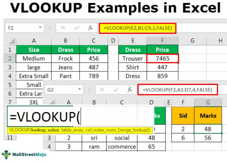
2. Type =VLOOKUP(, then fill in the function with your parameters:
   • Lookup_value: The value you want to search for.
   • Table_array: The range of cells that contain the data.
   • Col_index_num: The column number in the range containing the return value.
   • Range_lookup: TRUE for approximate match or FALSE for an exact match.
3. Press Enter to get your result.

Example:

=VLOOKUP(A2, Sheet2!A1:C100, 2, FALSE)

⚠️ Note: Remember that cell references in VLOOKUP will not automatically update when moving sheets between platforms. Double-check your references in Excel to ensure accuracy.

Overcoming Common Pitfalls

While VLOOKUP is straightforward, here are some common issues and how to address them:

• #N/A Error: This often occurs due to a mismatch in the lookup value or the lookup range not encompassing the entire dataset.
• Case Sensitivity: VLOOKUP is not case-sensitive, but if your data is, consider using EXACT or MATCH functions.
• Column Order: VLOOKUP looks in the first column of the range. Changing the order of columns requires redoing the function.

Enhancing VLOOKUP with Other Functions

To make VLOOKUP even more powerful, consider:

• IFERROR: Wrap VLOOKUP with IFERROR to handle errors gracefully.
• INDEX & MATCH: For more complex lookups or if you need to search across rows and columns.

Example:

=IFERROR(VLOOKUP(A2, Sheet2!A1:C100, 2, FALSE), “Not Found”)

The Power of Automation

If you’re dealing with regular updates or large datasets, automating the process can save time:

• Google Sheets Macros: Create macros to export sheets automatically to Excel format.
• Power Query: Excel’s Power Query can connect to Google Sheets, pulling in the latest data automatically.

Throughout this guide, we've covered how to integrate Google Sheets with Excel using VLOOKUP, ensuring a seamless transition and consistent data handling. By following these steps and tips, your data workflow will not only remain efficient but also become more precise. Whether you're analyzing small datasets or managing large projects, mastering this integration will elevate your productivity, giving you the confidence to manage data across platforms effortlessly. Integrating Google Sheets and Excel with VLOOKUP isn't just about using a function; it's about optimizing your data management strategy to save time and reduce errors, making your work life much easier.

Can I use VLOOKUP across different sheets?

+

Yes, VLOOKUP can work across different sheets within the same workbook. Simply reference the table array with the sheet name, like this: =VLOOKUP(value,Sheet2!A1:C100,2,FALSE).

Does VLOOKUP work with merged cells?

+

VLOOKUP does not work effectively with merged cells. The function looks for exact matches in the first column, which can become ambiguous with merged cells. It’s best to unmerge cells before using VLOOKUP.

What’s the difference between approximate and exact match in VLOOKUP?

+

An approximate match (TRUE or 1) finds the closest match if there’s no exact match, sorting the first column in ascending order. An exact match (FALSE or 0) looks for an exact match. If not found, it returns #N/A.